Home · Book Reports · 2018 · Mastering Machine Learning With Python in Six Steps

- Author :: Manohar Swamynathan
- Publication Year :: 2017
- Read Date :: 2018-03-16
- Source :: Mastering_Machine_Learning_with_Python_in_Six_Steps_-_1E_(2017).epub
designates my notes. / designates important.
Thoughts
After starting off on a great foot with a detailed table of contents and a chapter 1 that, while was merely an overview of python I breezed through, had a few bits of knowledge concerning dicts and sets I wasn’t aware of, things quickly took a turn for the worse.
First the not so bad. The algorithms, feature engineering, and general concepts are presented fairly well. I learned quite a bit, this being the first machine learning book I have read. There are plenty of diagrams to supplement the descriptions of the various techniques.
With the good out of the way…
The errors piled up example after example. The most common ’error’ was not including which imports were necessary. I spent a good deal of time online trying to figure out what I needed to import before the code would even try to run. Trying to see a silver lining, I consoled myself in the knowledge that by being forced to look up package after package, I was garnering a better understanding of what was available in the machine learning world.
After presenting a large section talking about pandas, numpy, and sklearn, the book takes another turn and starts using, unannounced and with no introduction I might add, statsmodels. As usual it also does so without telling you how to import it (import statsmodels.api as sm).
The function ‘plot_decision_regions()’ is used and not defined anywhere. I can not find library it is in but I did manage to find a few variations online, but they have different parameterization. Eventually I gave up on this one.
Last, and in this case certainly least egregious was the English, which is at time quite… “odd”. This, of course, can be excused. The missing code can not.
In conclusion, this was one of the worst programming books I have ever read. It was absolutely infuriating to work with the code examples. The programming independent machine learning information, on the other hand, was presented fairly clearly. In the end, I would not recommend it.
Interesting
One, somewhat random, observation that I would be interested to know more about is the fact that “clustering analysis origins can be traced to the area of Anthropology and Psychology in the 1930’s.” Given what my nontechnical research has revealed about these two fields, it might prove to be… insightful to understand the origins of clustering.
Code
This is the code I tinkered with, none of it should be considered usable in any way and is here merely for archival purposes.
- bagging.py
- boosting.py
- decision_tree_model.py
- diabetes_1.py
- doc_matrix.py
- generalized_linear_models.py
- google_word_model.py
- gradient_boost.py
- Housing.csv
- housing.py
- k_cluster.py
- k_folds.py
- k_nearest_neighbors.py
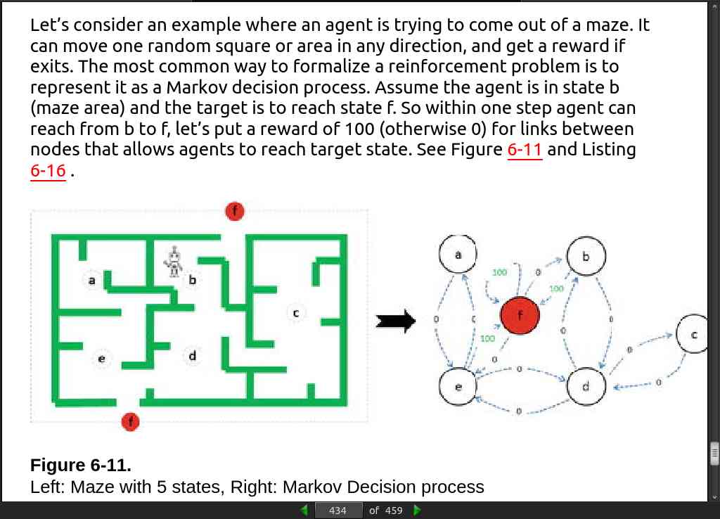
- markov_maze.py
- multiclass_logistic_regression.py
- multilayer_perceptron.py
- nonlinear_regression.py
- normalized.py
- perceptron.py
- principal_component_analysis.py
- svm_model.py
- test_grades.csv
- test_grades.py
- test_grades_2.csv
- test_grades_2.py
- test_grades_3.csv
- test_grades_3.py
Exceptional Excerpts
Table of Contents
- 01: Getting Started in Python
- 02: Introduction to Machine Learning
- 03: Fundamentals of Machine Learning
- 04: Model Diagnosis and Tuning
- 05: Text Mining and Recommender Systems
- 06: Deep and Reinforcement Learning
· 01: Getting Started in Python
page 15:
- I recommend Anaconda (Python distribution), which is BSD licensed and gives you permission to use it commercially and for redistribution. It has around 270 packages including the most important ones for most scientificapplications, data analysis, and machine learning…
page 049:

page 52:
# initialize A and B
A = {1, 2, 3, 4, 5}
B = {4, 5, 6, 7, 8}

# use | operator
print "Union of A | B", A|B

# alternative we can use union()
A.union(B)

---- output ----
Union of A | B set([1, 2, 3, 4, 5, 6, 7, 8])
Listing 1-33.
# use & operator
print "Intersection of A & B", A & B

# alternative we can use intersection()
print A.intersection(B)

---- output ----
Intersection of A & B set([4, 5])
Listing 1-34.
page 53:
# use - operator on A
print "Difference of A - B", A - B

# alternative we can use difference()
print A.difference(B)

---- output ----
Difference of A - B set([1, 2, 3])
Listing 1-35.
# use ^ operator
print "Symmetric difference of A ^ B", A ^ B

# alternative we can use symmetric_difference()
A.symmetric_difference(B)

---- output ----
Symmetric difference of A ^ B set([1, 2, 3, 6, 7, 8])
Listing 1-36.
page 56:
dict.get(key, default=None)
# returns None if key not present

dict[key]
# will error if key not present
dict.setdefault(key, default=None)
# adds a new key with default value
# like defaultdict?
page 64:
# Simple function to loop through arguments and print them
def sample_function(*args):
for a in args:
print a

# Call the function
Sample_function(1,2,3)
1
2
3

Listing 1-47.
# Simple function to loop through arguments and print them
def sample_function(**kwargs):
for a in kwargs:
print a, kwargs[a]

# Call the function
sample_function(name='John', age=27)
age 27
name 'John'

Listing 1-48.
· 02: Introduction to Machine Learning
page 75:
- Machine learning is a subfield of computer science that evolved from the study of pattern recognition…
page 76:
- AI process loop:
Observe – identify patterns using the data
Plan – find all possible solutions
Optimize – find optimal solution from the list of possible solutions
Action – execute the optimal solution
Learn and Adapt – is the result giving expected result, if no adapt

page 077:
page 079:
page 082:
page 83:
- “Knowledge Discovery in Databases” (KDD)
page 085:

page 87:
- Prescriptive analytic systems are a combination of business rules, machine learning algorithms, tools that can be applied against historic and real-time data feed. The key objective here is not just to predict what will happen, but also why it will happen…
page 88:
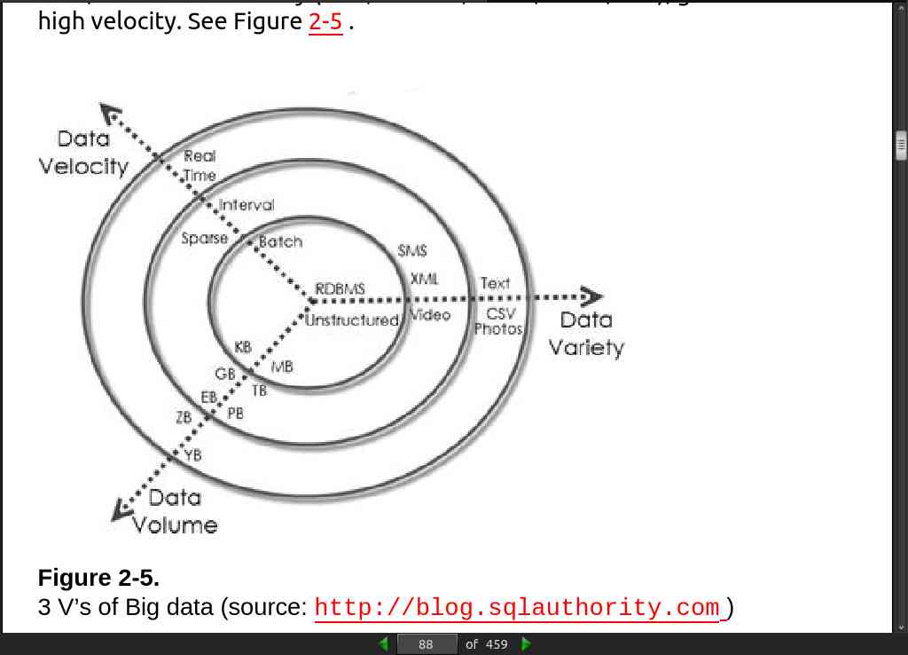
- As of 2008, the world’s servers processed 9.57 zeta-bytes (9.57 trillion gigabytes) of information, which is equivalent to 12 gigabytes of information per person per day, according to the “How Much Information? 2010 report on Enterprise Server Information.”
page 089:

page 090:
page 91:
- // Supervised learning, Regression or Classification.
page 92:
- // Unsupervised learning, Clustering, Dimension reduction, Anomaly detection, Reinforcement learning, (Markov, Q-learning, Temporal Difference, Monte-Carlo)
page 94:
- Knowledge Discovery Databases (KDD) This refers to the overall process of discovering useful knowledge from data…

page 097:
page 100:

page 101:
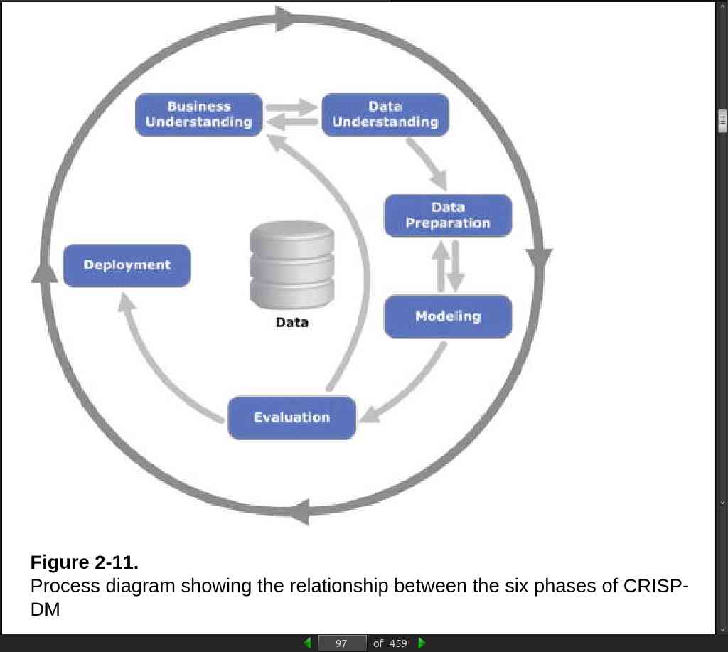
- In general most of the researchers and data mining experts follow the KDD and CRISP-DM process model because it is more complete and accurate.
page 102:

page 109:
- A slice of an [numpy] array is a view into the same data, so modifying it will modify the original array.
page 111:
a=np.array([[1,2], [3, 4], [5, 6]])

# Find the elements of a that are bigger than 2
print (a > 2)

# to get the actual value
print a[a > 2]

---- output ----
[[False False]
[ True True]
[ True True]]
[3 4 5 6]

Listing 2-8.
Boolean array indexing
page 114:
x=np.array([[1,2],[3,4]])

# Compute sum of all elements
print np.sum(x)

# Compute sum of each column
print np.sum(x, axis=0)

# Compute sum of each row
print np.sum(x, axis=1)

# ---- output ----
10
[4 6]
[3 7]

Listing 2-11.
Sum function
page 115:
-
Broadcasting
-
Broadcasting enables arithmetic operations to be performed between different shaped arrays. Let’s look at a simple example of adding a constant vector to each row of a matrix. See Listing 2-13.
# create a matrix
a = np.array([[1,2,3], [4,5,6], [7,8,9]])

# create a vector
v = np.array([1, 0, 1])

# create an empty matrix with the same shape as a
b = np.empty_like(a)

# Add the vector v to each row of the matrix x with an explicit loop
for i in range(3):
b[i, :] = a[i, :] + v
print b

# ---- output ----
[[ 2 2 4]
[ 5 5 7]
[ 8 8 10]]

Listing 2-13.
Broadcasting
- If you have to perform the above operation on a large matrix, the through loop in Python could be slow. Let’s look at an alternative approach. See Listing 2-14.
# Stack 3 copies of v on top of each other
vv = np.tile(v, (3, 1))
print vv

# ---- output ----
[[1 0 1]
[1 0 1]
[1 0 1]]

# Add a and vv elementwise
b = a + vvprint b

# ---- output ----
[[ 2 2 4]
[ 5 5 7]
[ 8 8 10]]

Listing 2-14.
Broadcasting for large matrix
- Now let’s see in Listing 2-15 how the above can be achieved using NumPy broadcasting.
a = np.array([[1,2,3], [4,5,6], [7,8,9]])
v = np.array([1, 0, 1])

# Add v to each row of a using broadcasting
b = a + v
print b

# ---- output ----
[[ 2 2 4]
[ 5 5 7]
[ 8 8 10]]

Listing 2-15.
Broadcasting using NumPy
- Now let’s look at some applications of broadcasting in Listing 2-16.
# Compute outer product of vectors
# v has shape (3,)
v = np.array([1,2,3])

# w has shape (2,)
w = np.array([4,5])

# To compute an outer product, we first reshape v to be a column
# vector of shape (3, 1); we can then broadcast it against w to yield
# an output of shape (3, 2), which is the outer product of v and w:
print np.reshape(v, (3, 1)) * w

# ---- output ----
[[ 4 5]
[ 8 10]
[12 15]]

# Add a vector to each row of a matrix
x = np.array([[1,2,3],[4,5,6]])

# x has shape (2, 3) and v has shape (3,) so they
broadcast to (2, 3)
printx + v

# ---- output ----
[[2 4 6]
[5 7 9]]

# Add a vector to each column of a matrix
# x has shape (2, 3) and w has shape (2,).
# If we transpose x then it has shape (3, 2) and can be broadcast
# against w to yield a result of shape (3, 2); transposing this result
# yields the final result of shape (2, 3) which is the matrix x with
# the vector w added to each column
print(x.T + w).T

# ---- output ----
[[ 5 6 7]
[ 9 10 11]]

# Another solution is to reshape w to be a row vector of shape (2, 1);
# we can then broadcast it directly against x to produce the same
# output.
printx + np.reshape(w,(2,1))

# ---- output ----
[[ 5 6 7]
[ 9 10 11]]

# Multiply a matrix by a constant:
# x has shape (2, 3). Numpy treats scalars as arrays ofshape ();
# these can be broadcast together to shape (2, 3)
printx * 2

# ---- output ----
[[ 2 4 6]
[ 8 10 12]]

Listing 2-16.
Applications of broadcasting
page 118:
-
Broadcasting typically makes your code more concise and faster, so you should strive to use it where possible.
-
// Pandas section
page 133:
- // Matplotlib section
page 152:
- Scikit-learn is the most popular and widely used machine learning library. It is built on top of SciPy and features a rich number of supervised and unsupervised learning algorithms.
· 03: Fundamentals of Machine Learning
page 154:
- Statsmodels: This complements the SciPy package and is one of the best packages to run regression models as it provides an extensive list of statistics results for each estimator of the model.
page 157:
page 158:
- // Ways to deal with missing data.
Delete
Replace (mean/mode)
Random
Predictive model
page 161:

page 177:

page 211:
page 226:

page 230:
- SVM is comparatively less prone to outliers than logistic regression as it only cares about the points that are closest to the decision boundary or support vectors.

page 233:
- // plot_decision_regions() is a total mystery function.
page 236:
- Decision Trees, SVM, and kNNbase algorithm concepts can essentially be applied to predict dependent variables that are continuous numbers in nature, and Scikit-learn provides DecisionTreeRegressor, SVR (support vector regressor), and kNeighborsRegressor for the same.
page 247:
- Clustering analysis origins can be traced to the area of Anthropology and Psychology in the 1930’s.
page 249:
-
Limitations of K-means:
-
K-means clustering needs the number of clusters to be specified.
-
K-means has problems when clusters are of differing sized, densities, and non-globular shapes.
-
Presence of outlier can skew the results.
page 258:

page 265:
{{ exclamation(“summary”) }}
- Supervised models such as linear and nonlinear regression techniques are useful to model patterns to predict continuous numerical data types. Whereas logistic regression, decision trees, SVM and kNN are useful to model classification problems (functions are available to use for regression as well).You also learned ARIMA, which is one of the key time-series forecasting models. Unsupervised techniques such as k-means and hierarchical clustering are useful to group similar items, whereas principal component analysis can be used to reduce a large dimension data to lower a dimension to enable efficient computation.
· 04: Model Diagnosis and Tuning
page 266:
- Throughout this chapter, we’ll mostly be using a dataset from the UCI repository, “Pima Indian diabetes,” which has 768 records, 8 attributes, 2 classes, 268 (34.9%) positive results for diabetes test, and 500 (65.1%) negative results.
page 271:

page 272:
-
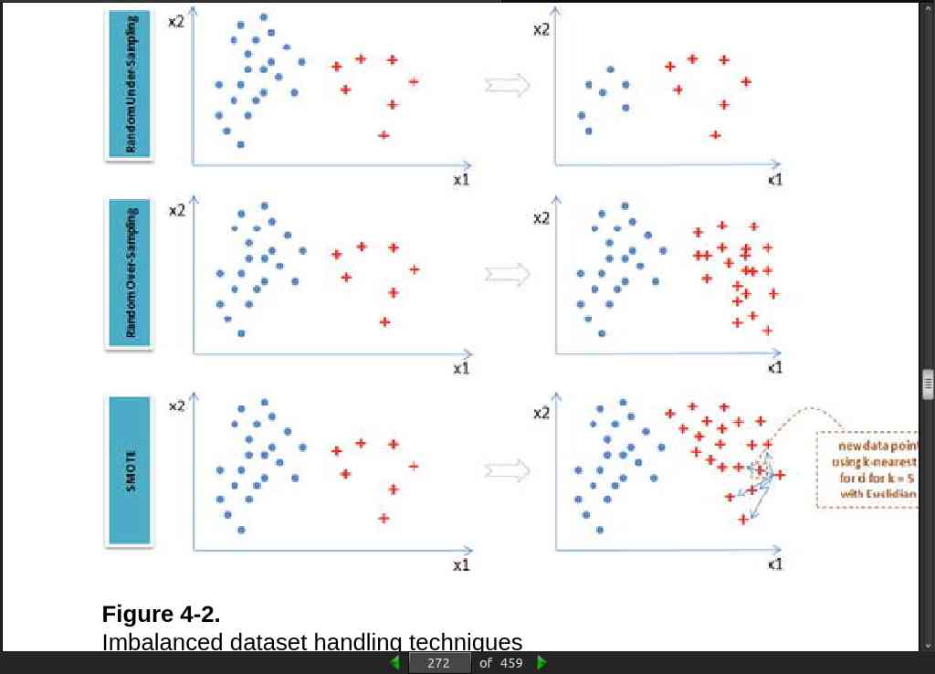
Providing an equal sample of positive and negative instances to the classification algorithm will result in an optimal result. Datasets that are highly skewed toward one or more classes have proven to be a challenge.
-
// Without enough samples you have several options:
-
Random under-sampling – Reduce majority class to match minority class count.
-
Random over-sampling – Increase minority class by randomly picking samples within minority class till counts of both class match.
-
Synthetic Minority Over-Sampling Technique (SMOTE) – Increase minority class by introducing synthetic examples through connecting all k (default = 5) minority class nearest neighbors using feature space similarity (Euclidean distance). See Figure 4-2 .
page 275:
-
Random Under-Sampling raises the opportunity for loss of information or concepts as we are reducing the majority class.
-
Random Over-Sampling and SMOTE can lead to over-fitting issues due to multiple related instances.
page 277:
-
If model accuracy is low on a training dataset as well as test dataset the model is said to be under-fitting or that the model has high bias.
-
If a model is giving high accuracy on a training dataset, however on a test dataset the accuracy drops drastically, then the model is said to be over fitting or a model that has high variance.
-
// I am pretty much giving up on the demo code at this point. Literally 90% of the code fails because it doesn’t tell you what to import etc. This has to be the worst programming book I have ever read, hands down.
page 278:

page 279:
page 290:
page 293:
· 05: Text Mining and Recommender Systems
page 318:

page 319:
page 320:
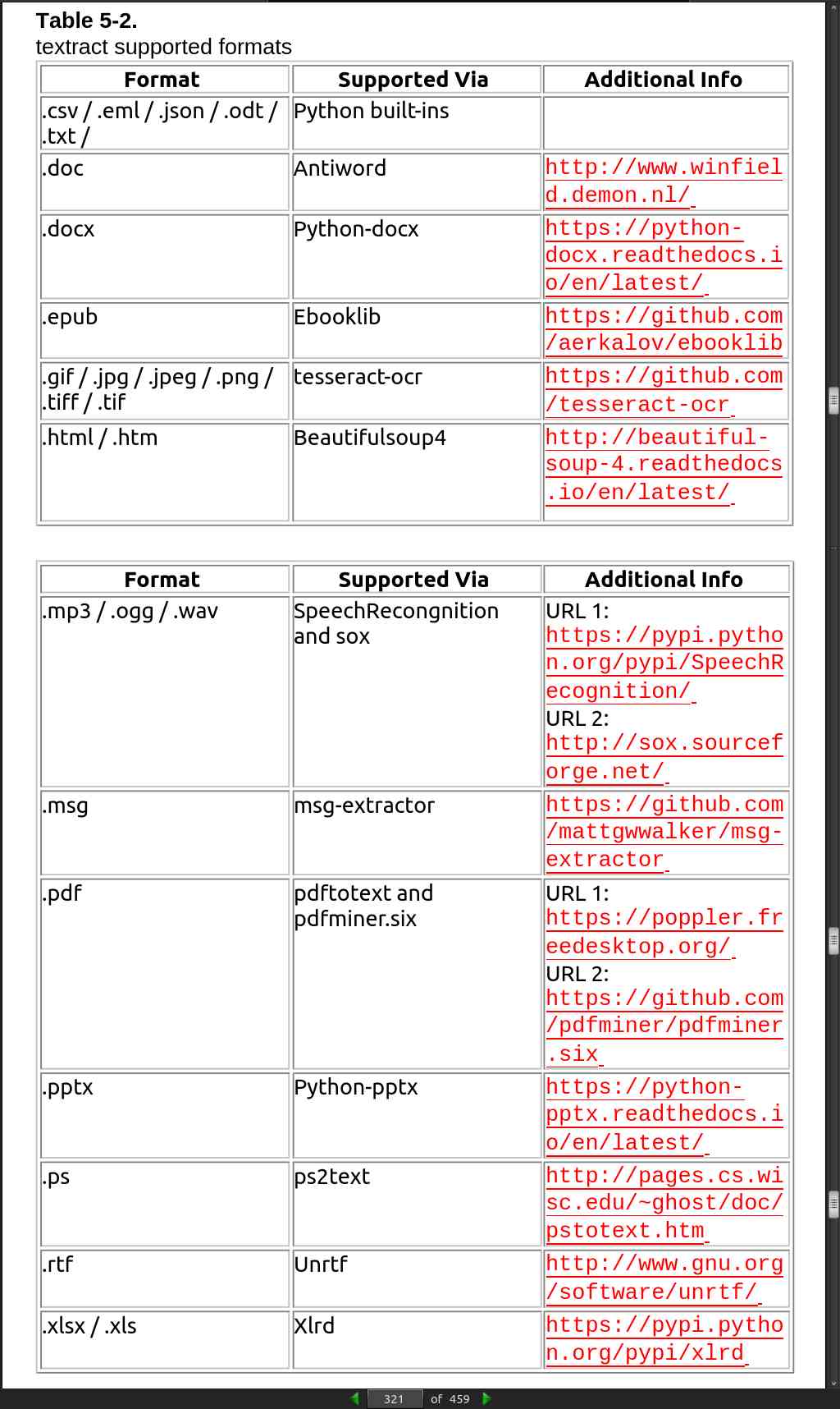
- There are several libraries available for extracting text content from different formats discussed above. By far the best library that provides a simple and single interface for multiple formats is ‘textract’ (open source MIT license).
page 320:
page 366:
-
You can download Google’s pre-trained model (from given link below) for word2vec, which includes a vocabulary of 3 million words/phrases taken from 100 billion words from a Google News dataset.
-
URL: https://drive.google.com/file/d/0B7XkCwpI5KDYNlNUTTlSS21pQmM/edit
· 06: Deep and Reinforcement Learning
page 376:
page 377:

page 380:
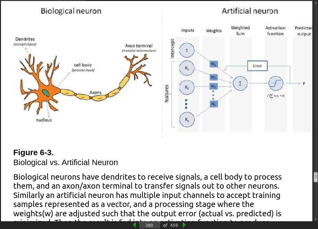
page 383:

page 385:
-
Multilayer Perceptrons (Feedforward Neural Network)
-
hidden_layer_sizes – You have to provide the number of hidden layers and neurons for each hidden layer. For example, hidden_layer_sizes – (5,3,3) means there are 3 hidden layers and the number of neurons for layer 1 is 5, layer 2 is 3, and for layer 3 is 3 respectively. The default value is (100,) that is, 1 hidden layer with 100 neurons.
-
Activation – This is the activation function for hidden layer, and there are four activation functions available for use, default is ‘relu’.
-
relu: The rectified linear unit function, returns f(x) = max(0, x).
-
logistic: The logistic sigmoid function, returns f(x) = 1 / (1 + exp(-x)).
-
identity: No-op activation, useful to implement linear bottleneck, returns f(x) = x.
-
tanh: The hyperbolic tan function, returns f(x) = tanh(x).
-
solver – This is for weight optimization’ there are three options available,the default being ‘adam’.
-
adam: Stochastic gradient-based optimizer proposed by Kingma/Diederik/Jimmy Ba, which works well for large dataset.
-
lbfgs: Belongs to family of quasi-Newton methods, works well for small datasets.
-
sgd: Stochastic gradient descent.
-
max_iter – This is the maximum number of iterations for solver to converge, default is 200.
-
learning_rate_init – This is the initial learning rate to control step size for updating the weights (only applicable for solvers sgd/adam), default is 0.001.
page 422:
- The MLP (feedforward network) is not known to do well on sequential events models such as the probabilistic language model of predicting the next word based on the previous word at every given point. Recurrent Neural Network (RNN) architecture addresses this issue. It is similar to MLP except that they have a feedback loop, which means they feed previous time steps into the current step. This type of architecture generates sequences to simulate situation and create synthetic data, making them the ideal modeling choice to work on sequence data such as speech text mining, image captioning, time series prediction, robot control, language modeling, etc.
page 423:
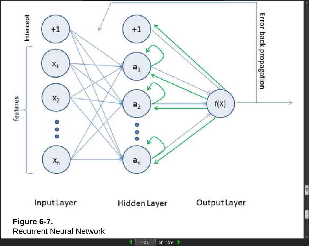
page 424:
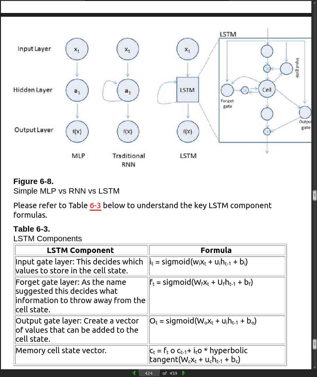
page 434:
