Home · Book Reports · 2017 · Fundamentals of Electrical Engineering I

---

---

---

---

designates my notes. / designates important.

---

Thoughts

Heavy focus on signals and systems theory over “practical” electronics. I would not suggest this as a first course if you are interested in EE/EECS. If you are looking for communications theory, this is perfect.

IMHO the 2007 MIT 6.002 Circuits and Electronics is a better place to start. Further, the 2011 MIT 6.01SC was also more appealing to me as it mixes the theory with a more hands on approach (python programming and robots). The next course in this Rice U series, ELEC242 I think, looks good but is not available online.

---

• ELEC 241 at Rice.edu

• There are lectures for this online, if you can find them.

• CONNEXIONS, Rice University, Houston, Texas

• pdf page numbers

---

Table of Contents

• Chapter 1 - Introduction
• Chapter 2 - Signals and Systems
• Chapter 3 - Analog Signal Processing
• Chapter 4 - Frequency Domain
• Chapter 5 - Digital Signal Processing
• Chapter 6 - Information Communication

---

· Chapter 1 - Introduction

page 7:

• The conversion of information-bearing signals from one energy form into another is known as energy conversion or transduction.

page 8:

• A Mathematical Theory of Communication by Claude Shannon (1948)

• a signal is merely a function. Analog signals are continuous- valued; digital signals are discrete-valued. The independent variable of the signal could be time (speech, for example), space (images), or the integers (denoting the sequencing of letters and numbers in the football score)

page 8:

• The basic idea of communication engineering is to use a signal’s parameters to represent either real numbers or other signals. The technical term is to modulate the carrier signal’s parameters to transmit information

· Chapter 2 - Signals and Systems

page 17:

• The complex conjugate of z, written as z∗

page 18:

• multiplying a complex number by j rotates the number’s position by 90 degrees.

• polar form for complex numbers.

z = a + jb = r∠θ
r = |z| = √(a2 + b2)
a = r cos (θ)
b = r sin (θ)
θ = arctan(b/a)

• the polar form of a complex number z can be expressed mathematically as:

z = re^(jθ)

page 21:

• The complex exponential cannot be further decomposed into more elemental signals, and is the most important signal in electrical engineering

page 22:

• T = 1/f

• f = The number of times per second we go around the circle equals the frequency f.

• T = period, how long for one complex exponential cycle

These two decompositions are mathematically equivalent to each other.

A*cos(2πft + φ) = Re[Ae^(jφ)e^(j2πft)]
A*sin(2πft + φ) = Im[Ae^(jφ)e^(j2πft)]

page 23:

• As opposed to complex exponentials which oscillate, real exponentials (Figure 2.3) decay.

s(t) = e^(−t/τ)

• The quantity τ is known as the exponential’s time constant, and corresponds to the time required for the exponential to decrease by a factor of 1 , which approximately equals 0.368. A decaying complex exponential is the product of a real and a complex exponential.

page 24:

• ways of decomposing a given signal into a sum of simpler signals, which we term the signal decomposition

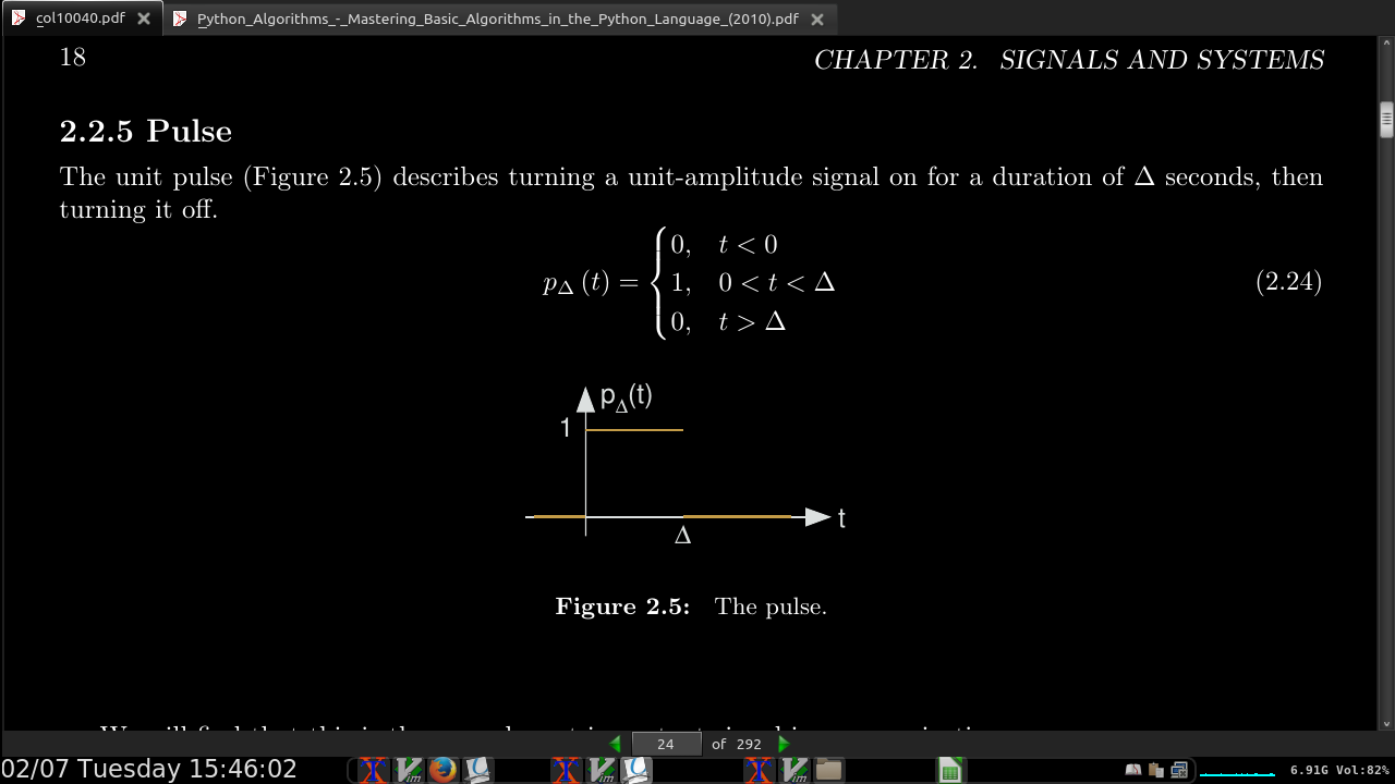
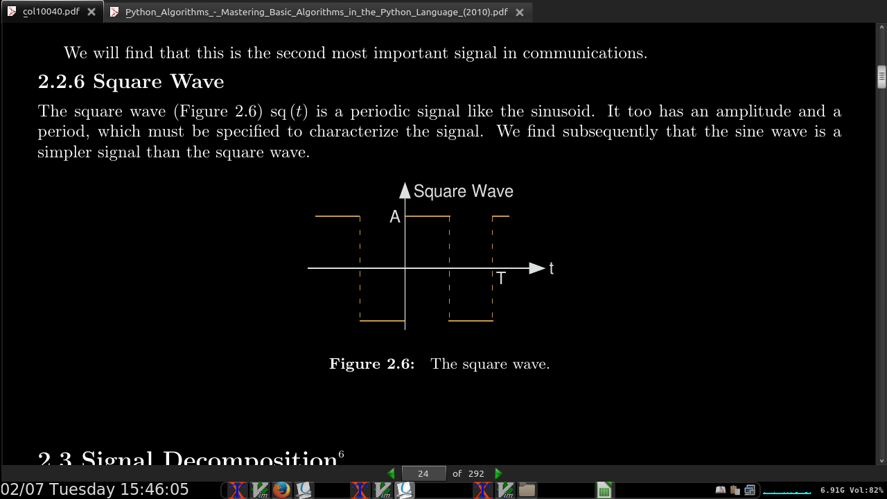
page 25:

• One of the fundamental results of signal theory (Section 5.3) will detail conditions under which an analog signal can be converted into a discrete-time one and retrieved without error.

• A discrete-time signal is represented symbolically as s (n), where n = {…,−1,0,1,…}.

page 26:

• The most important signal is, of course, the complex exponential sequence. s(n) = e^(j2πfn)

• Discrete-time sinusoids have the obvious form s(n) = A*cos(2πfn + φ).

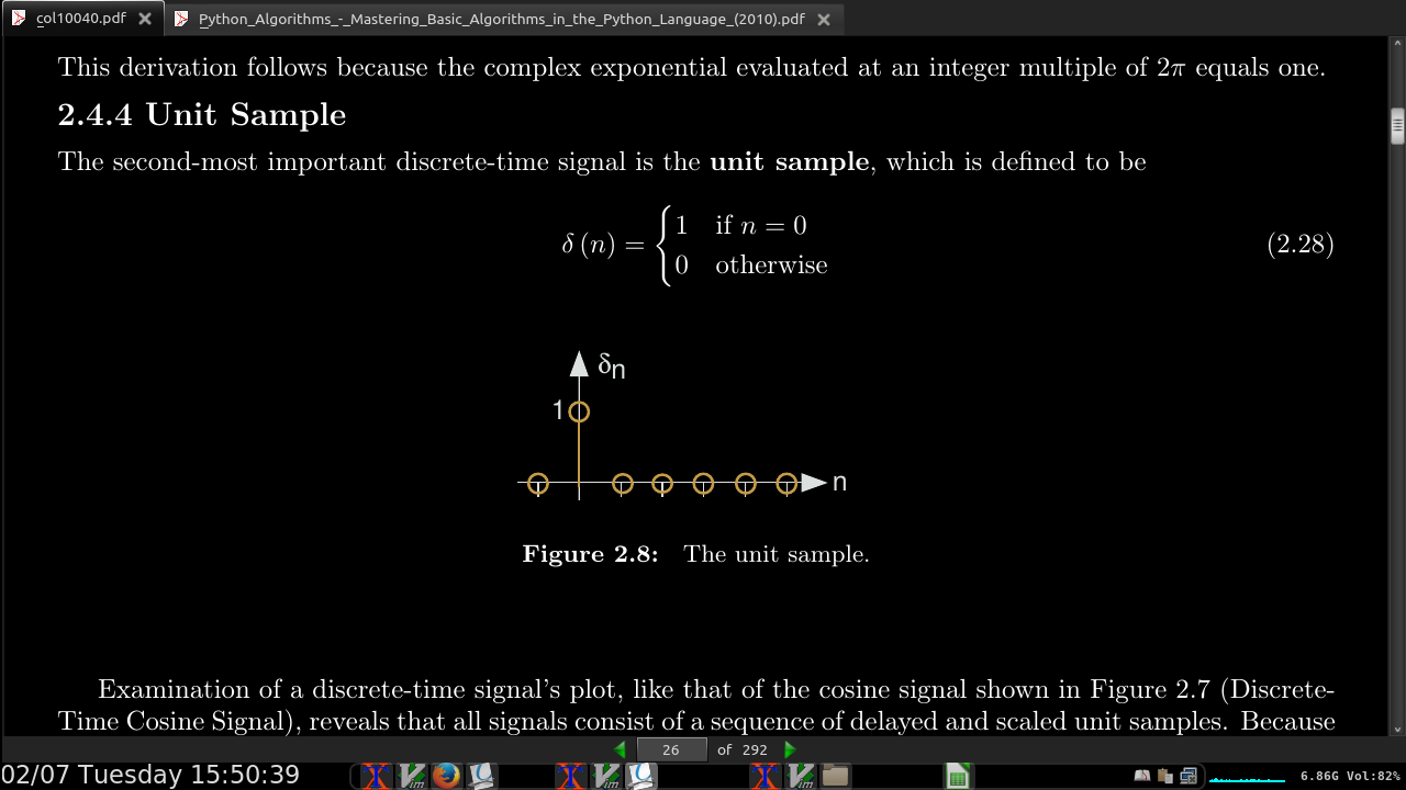
• all signals consist of a sequence of delayed and scaled unit samples.

• we can decompose any signal as a sum of unit samples delayed to the appropriate location and scaled by the signal value.

        ∞ 
s(n) = sum  s(m)δ(n − m)
       m=−∞
 

page 27:

• Another interesting aspect of discrete-time signals is that their values do not need to be real numbers. We do have real-valued discrete-time signals like the sinusoid, but we also have signals that denote the sequence of characters typed on the keyboard. Such characters certainly aren’t real numbers,

• like a math set, formally called alphabet (but not limited to characters in any actual language alphabet)

• discrete-time systems are ultimately constructed from digital circuits, which consist entirely of analog circuit elements.

• Signals are manipulated by systems. Mathematically, we represent what a system does by the notation y(t) = S[x(t)], with x representing the input signal and y the output signal.

• A system’s input is analogous to an independent variable and its output the dependent variable. For the mathematically inclined, a system is a functional: a function of a function (signals are functions).

• Systems can be linked like linux pipes

• w(t) = S1[x(t)], and y(t) = S2[w(t)]

page 28:

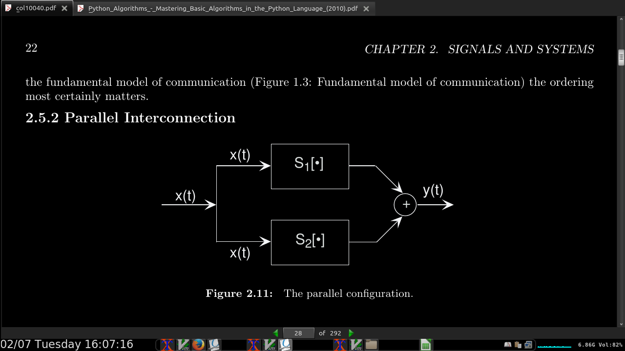
• y(t) = S1[x(t)] + S2[x(t)]

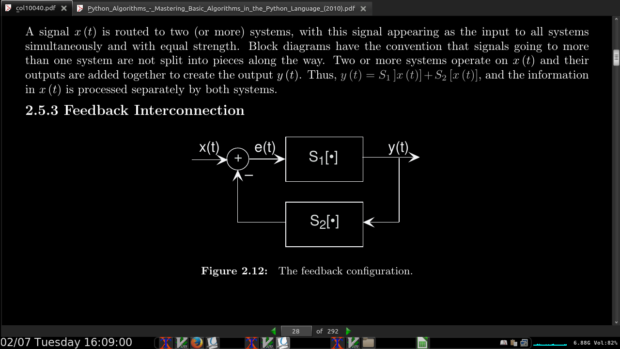
• y(t) = S1[e(t)]

• The input e(t) equals the input signal minus the output of some other system’s output to y(t): e(t) = x(t) − S2[y(t)].

page 29:

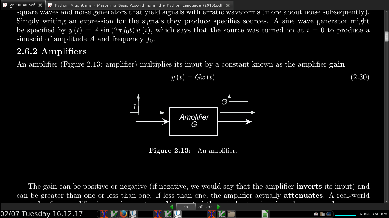
• The gain can be positive or negative (if negative, we would say that the amplifier inverts its input) and can be greater than one or less than one. If less than one, the amplifier actually attenuates.

page 30:

• Derivative system y(t) = dx/dt(t)

• Integratort

          t
y(t) = integral x(α)dα
          −∞

• the value of all signals at t = −∞ equals zero.

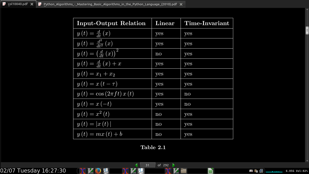
• linear systems, double the input double the output as a simple test (not 100%)

• linear systems output 0 on input 0

page 31:

• “They’re [linear systems] the only systems we thoroughly understand!”

• Systems that don’t change their input-output relation with time are said to be time-invariant.

• The collection of linear, time-invariant systems are the most thoroughly understood systems

• electric circuits are, for the most part, linear and time-invariant. Nonlinear ones abound, but characterizing them so that you can predict their behavior for any input remains an unsolved problem.

· Chapter 3 - Analog Signal Processing

page 39:

• When we say that “electrons flow through a conductor,” what we mean is that the conductor’s constituent atoms freely give up electrons from their outer shells. “Flow” thus means that electrons hop from atom to atom driven along by the applied electric potential.

• A missing electron, however, is a virtual positive charge. Electrical engineers call these holes, and in some materials, particularly certain semiconductors, current flow is actually due to holes.

• Current flow also occurs in nerve cells found in your brain. Here, neurons “communicate” using propagating voltage pulses that rely on the flow of positive ions (potassium and sodium primarily, and to some degree calcium) across the neuron’s outer wall.

page 40:

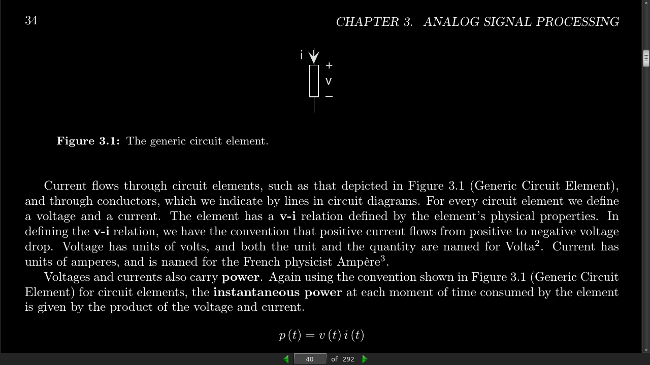
• For every circuit element we define a voltage and a current. The element has a v-i relation defined by the element’s physical properties. In defining the v-i relation, we have the convention that positive current flows from positive to negative voltage drop.

• p(t) = v(t)i(t) (p)ower is measured in watts./span>

• A positive value for power indicates that at time t the circuit element is consuming power; a negative value means it is producing power.

• as in all areas of physics and chemistry, power is the rate at which energy is consumed or produced. Consequently, energy is the integral of power.

          t
E(t) =integral p(α)dα
          −∞

• positive energy corresponds to consumed energy and negative energy corresponds to energy production.

• —the resistor, capacitor, and inductor— impose linear relationships between voltage and current.

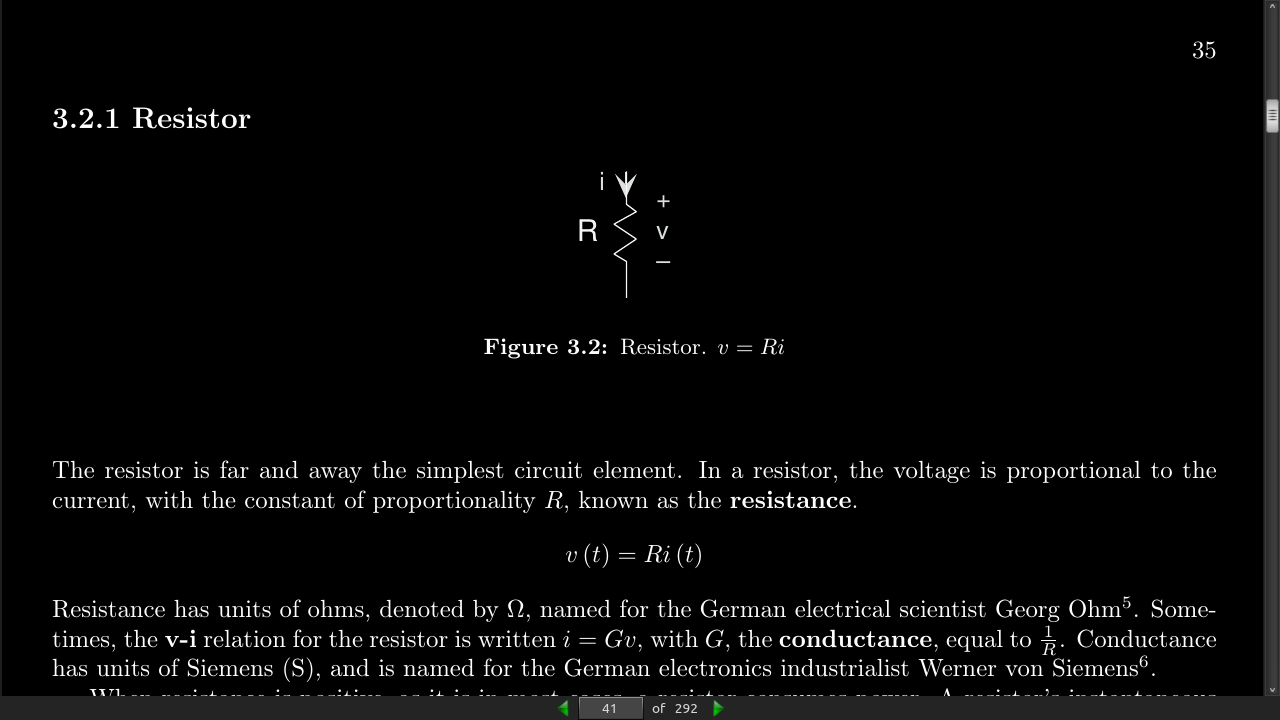
• v(t) = Ri(t)

page 41:

• Some- times, the v-i relation for the resistor is written i = Gv, with G, the conductance, equal to 1/R. Conductance Rhas units of Siemens (S)

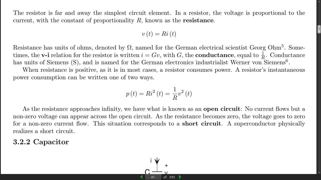
p(t) = Ri^2(t) = v^2(t)/R Instantaneous power consumption of a resistor.

• As the resistance approaches infinity, we have what is known as an open circuit: No current flows but a non-zero voltage can appear across the open circuit. As the resistance becomes zero, the voltage goes to zero for a non-zero current flow. This situation corresponds to a short circuit. A superconductor physically realizes a short circuit.

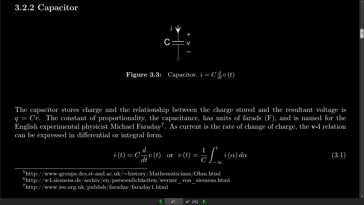
• The capacitor stores charge and the relationship between the charge stored and the resultant voltage is q = Cv. The constant of proportionality, the capacitance, has units of farads (F),

• As current is the rate of change of charge, the v-i relation can be expressed in differential or integral form.

page 42:

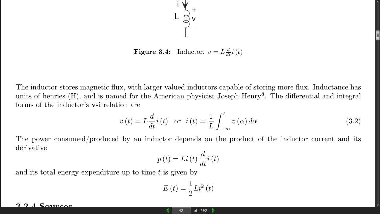
• The inductor stores magnetic flux, with larger valued inductors capable of storing more flux. Inductance has units of henries (H),

page 43:

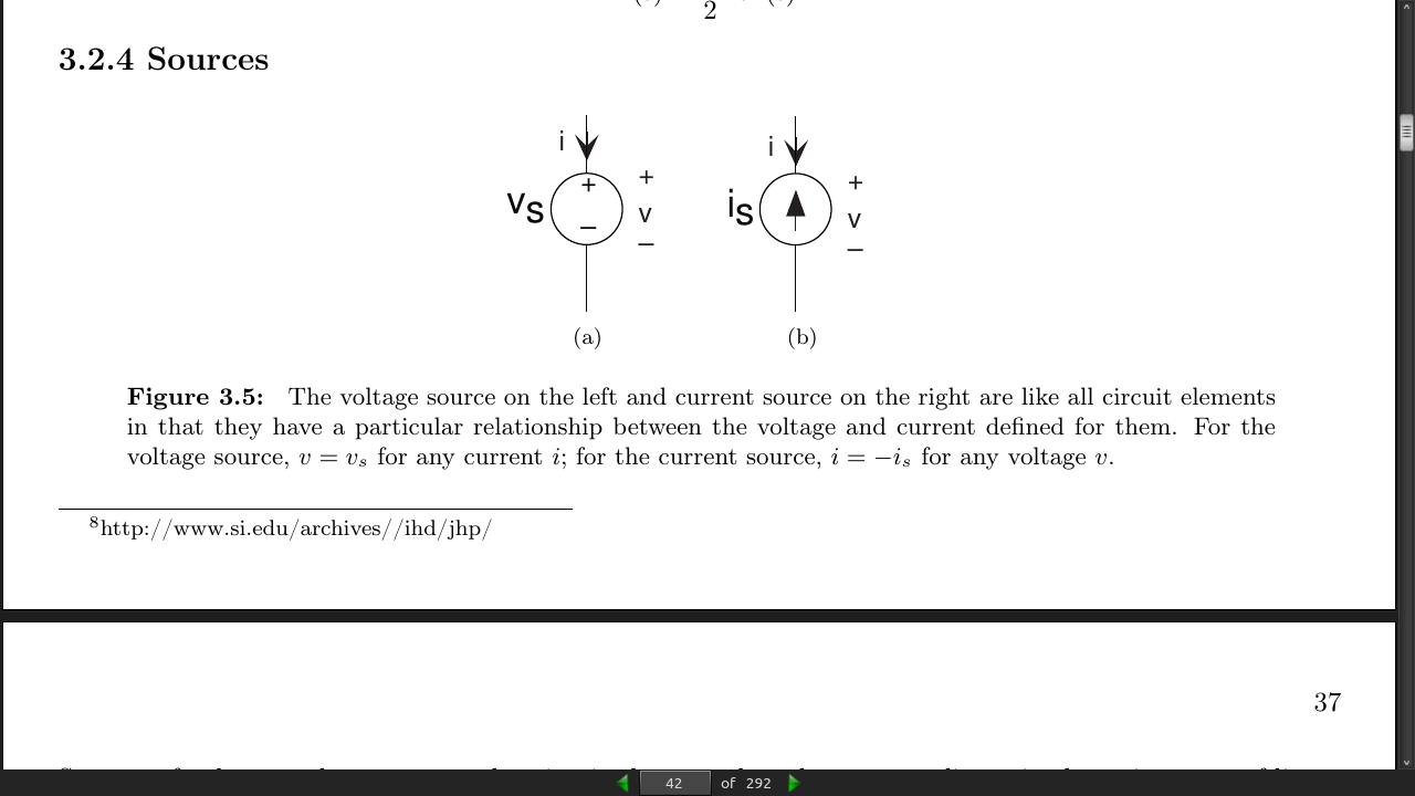
• voltage source’s v-i relation is v = vs regardless of what the current might be. As for the current source, i = −is regardless of the voltage. Another name for a constant-valued voltage source is a battery,

• If a sinusoidal voltage is placed across a physical resistor, the current will not be exactly proportional to it as frequency becomes high, say above 1 MHz. At very high frequencies, the way the resistor is constructed introduces inductance and capacitance effects. Thus, the smart engineer must be aware of the frequency ranges over which his ideal models match reality well.

page 44:

• Kirchhoff’s Current Law (KCL): At every node, the sum of all currents entering a node must equal zero.

• Kirchhoff’s Voltage Law (KVL): The voltage law says that the sum of voltages around every closed loop in the circuit must equal zero.</span

page 48:

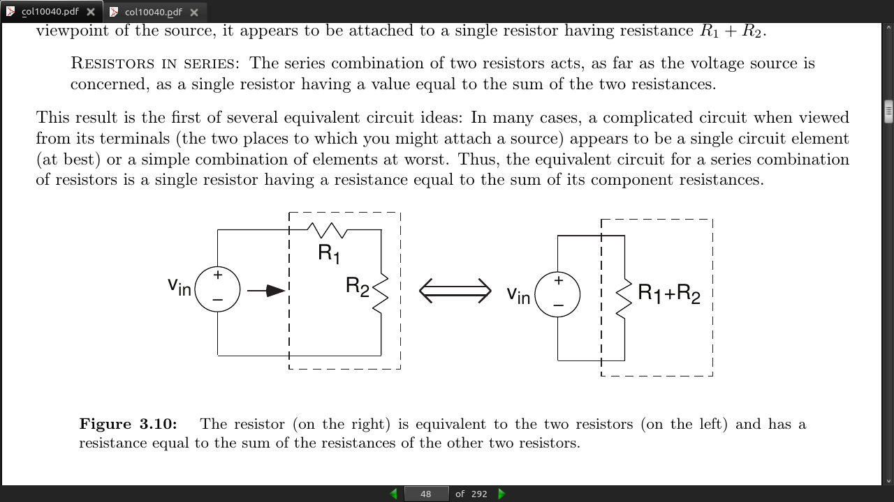
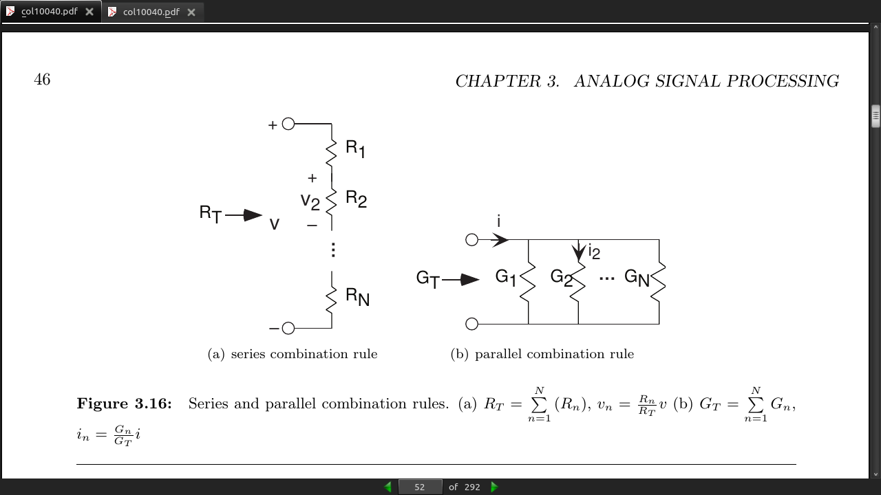
• Resistors in series: The series combination of two resistors acts, as far as the voltage source is concerned, as a single resistor having a value equal to the sum of the two resistances.

page 49:

page 51:

• Note that in determining this structure [//of series/parallel relationships//], we started away from the terminals, and worked toward them. In most cases, this approach works well; try it first.

RT = R1 || (R2 || R3 + R4)

RT = (R1*R2*R3 + R1*R2*R4 + R1*R3*R4) / (R1*R2 + R1*R3 + R2*R3 + R2*R4 + R3*R4)

• A simple check for accuracy is the units: Each component of the numerator should have the same units (here Ω^3 ) as well as in the denominator (Ω^2). The entire expression is to have units of resistance; thus, the ratio of the numerator’s and denominator’s units should be ohms.

• In system theory, systems can be cascaded without changing the input-output relation of intermediate systems. In cascading circuits, this ideal is rarely true unless the circuits are so designed.

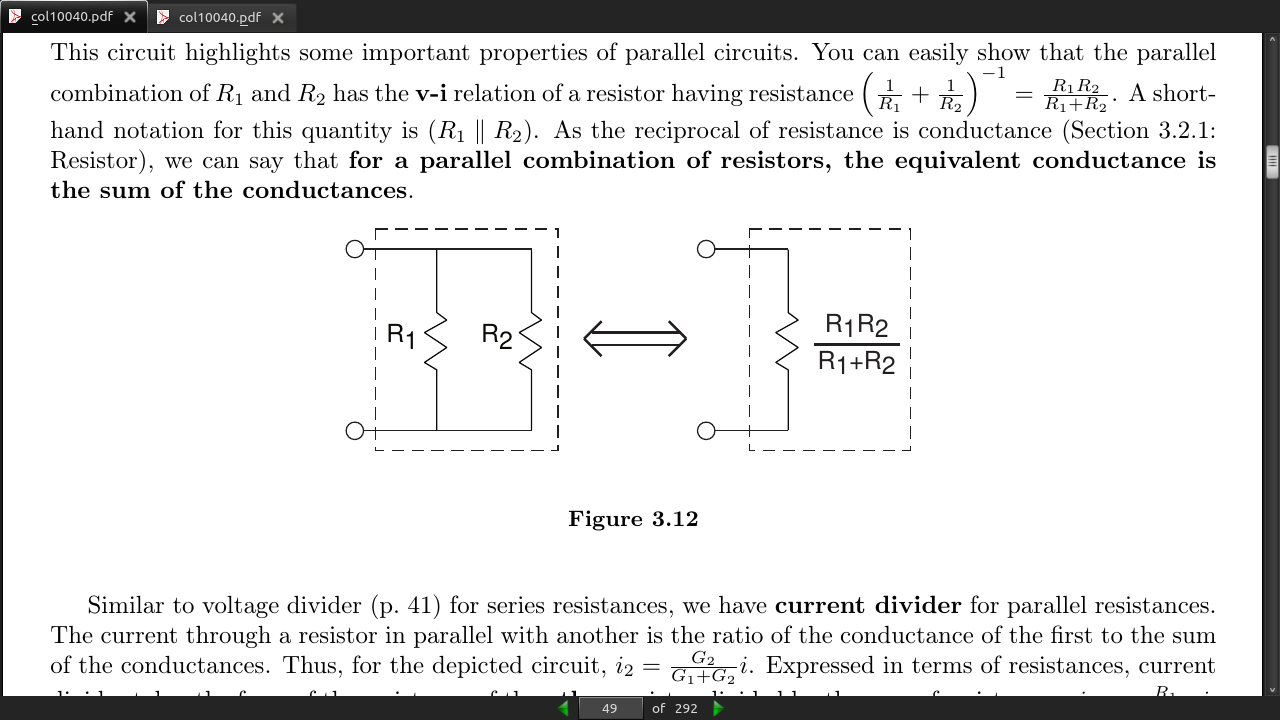
• for series combinations, voltage and resistance are the key quantities, while for parallel combinations current and conductance are more important. In series combinations, the currents through each element are the same; in parallel ones, the voltages are the same.

page 53:

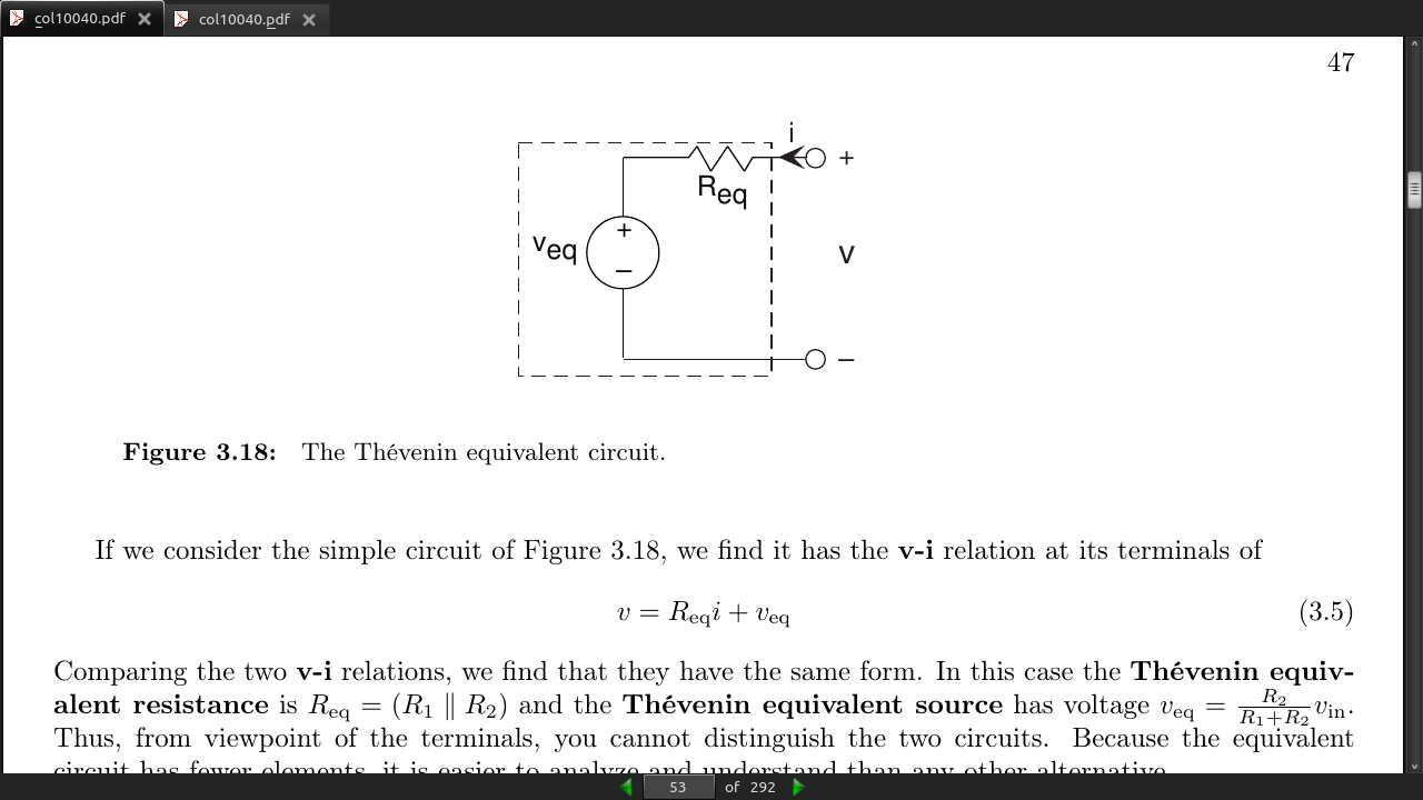
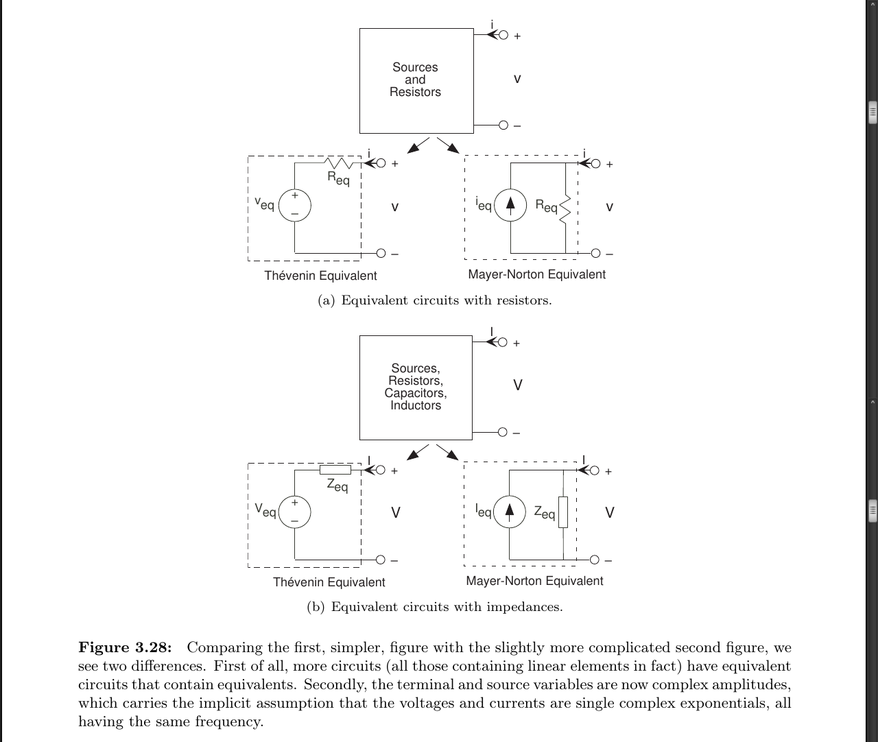
• For any circuit containing resistors and sources, the v-i relation will be of the form: v = R_eq*i + v_eq and is the Thévenin equivalent circuit for any such circuit is that of Figure 3.18.

page 55:

• Mayer-Norton equivalent: i = v/R_eq - i_eq, where i_eq = v_eq/R_eq is the Mayer-Norton equivalent source.

page 56:

• Which one is used depends on whether what is attached to the terminals is a series configuration (making the Thévenin equivalent the best) or a parallel one (making Mayer-Norton the best).

page 58:

• Because complex amplitudes for voltage and current also obey Kirchhoff’s laws, we can solve circuits using voltage and current divider and the series and parallel combination rules by considering the elements to be impedances.

• The entire point of using impedances is to get rid of time and concentrate on frequency.

page 59:

1. Even though it’s not, pretend the source is a complex exponential. We do this because the impedance approach simplifies finding how input and output are related. If it were a voltage source having voltage vin = p (t) (a pulse), still let vin = Vinej2πf t. We’ll learn how to “get the pulse back” later.

2. With a source equaling a complex exponential, all variables in a linear circuit will also be complex exponentials having the same frequency. The circuit’s only remaining “mystery” is what each variable’s complex amplitude might be. To find these, we consider the source to be a complex number (Vin here) and the elements to be impedances.

3. We can now solve using series and parallel combination rules how the complex amplitude of any variable relates to the sources complex amplitude.

page 60:

• Example 3.3 Good explaination of using impedence.

page 62:

• V_out/V_in = H(f) Transfer Function

• Implicit in using the transfer function is that the input is a complex exponential, and the output is also a complex exponential having the same frequency.

page 63:

• the transfer function completely describes how the circuit processes the input complex exponential to produce the output complex exponential. The circuit’s function is thus summarized by the transfer function. In fact, circuits are often designed to meet transfer function specifications.

page 64:

• magnitude has even symmetry: The negative frequency portion is a mirror image of the positive frequency portion: |H(−f)| = |H(f)|. The phase has odd symmetry: ∠H(−f) = −∠H(f). These properties of this specific example apply for all transfer functions associated with circuits.

page 67:

• The node method begins by finding all nodes–places where circuit elements attach to each other–in the circuit. We call one of the nodes the reference node; the choice of reference node is arbitrary, but it is usually chosen to be a point of symmetry or the “bottom” node. For the remaining nodes, we define node voltages e_n that represent the voltage between the node and the reference. These node voltages constitute the only unknowns; all we need is a sufficient number of equations to solve for them. In our example, we have two node voltages. The very act of defining node voltages is equivalent to using all the KVL equations at your disposal.

• In some cases, a node voltage corresponds exactly to the voltage across a voltage source. In such cases, the node voltage is specified by the source and is NOT an unknown.

page 68:

• A little reflection reveals that when writing the KCL equations for the sum of currents leaving a node, that node’s voltage will always appear with a plus sign, and all other node voltages with a minus sign. Systematic application of this procedure makes it easy to write node equations and to check them before solving them. Also remember to check units at this point.

page 72:

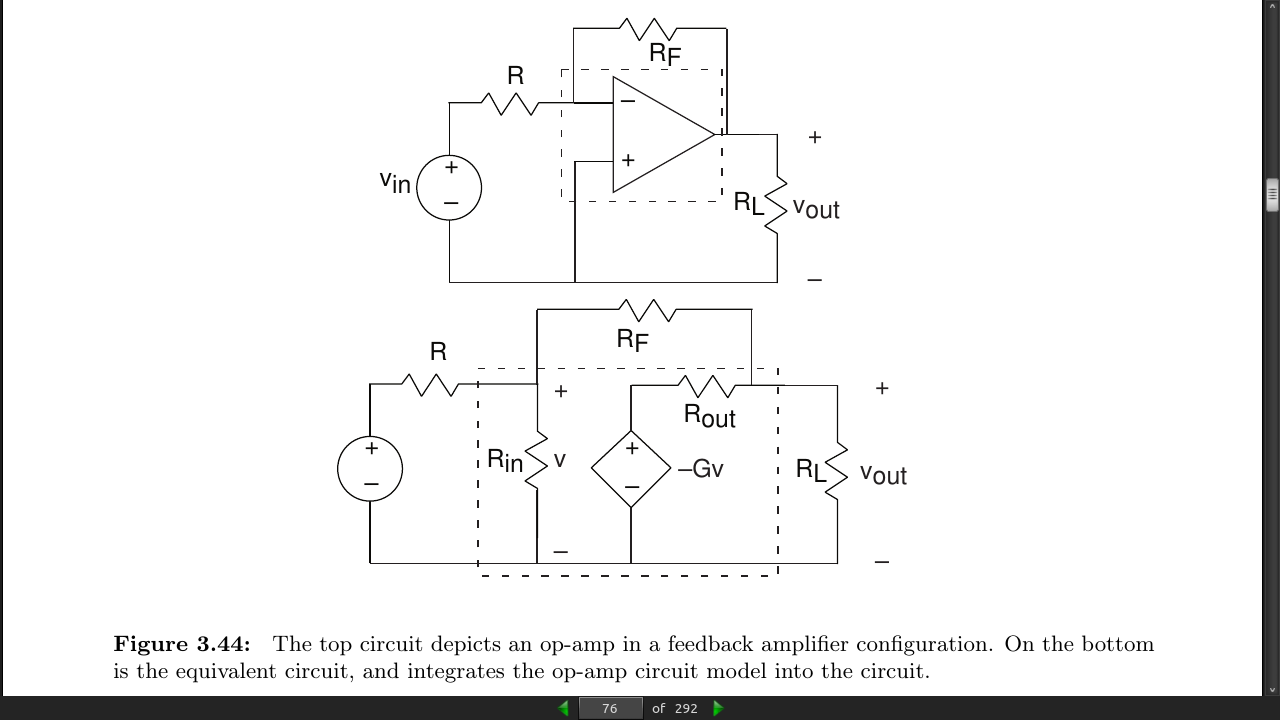
• Resistors, inductors, and capacitors as individual elements certainly provide no power gain, and circuits built of them will not magically do so either. Such circuits are termed electrical in distinction to those that do provide power gain: electronic circuits.

page 74:

• dependent sources cannot be described as impedances

page 80:

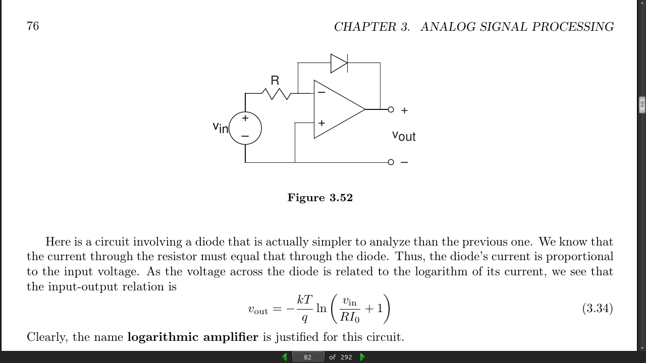
• i(t) = I_0 · e^(q/kT)*v(t) − 1

• q represents the charge of a single electron in coulombs, k is Boltzmann’s constant, and T is the diode’s temperature in K. At room temperature, the ratio kT/q = 25 mV. The constant I_0 is the qleakage current, and is usually very small

• diode’s schematic symbol looks like an arrowhead; the direction of current flow corresponds to the direction the arrowhead points.

• Because of the diode’s nonlinear nature, we cannot use impedances nor series/parallel combination rules to analyze circuits containing them.

page 82:

unsorted:

· Chapter 4 - Frequency Domain

page 107:

• all signals can be expressed as a superposition of sinusoids

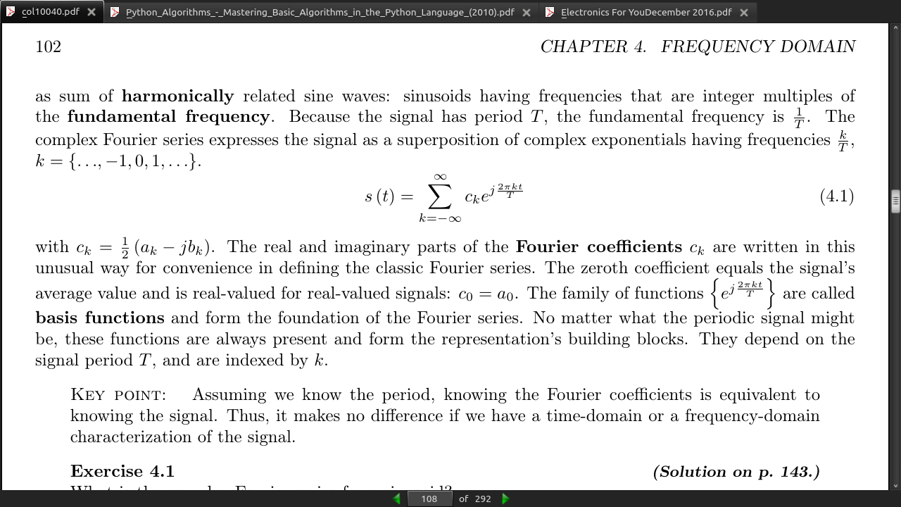
• Let s(t) be a periodic signal with period T. We want to show that periodic signals, even those that have constant-valued segments like a square wave, can be expressed as sum of harmonically related sine waves: sinusoids having frequencies that are integer multiples of the fundamental frequency. Because the signal has period T, the fundamental frequency is 1/T.

page 108:

• Key point: Assuming we know the period, knowing the Fourier coefficients is equivalent to knowing the signal. Thus, it makes no difference if we have a time-domain or a frequency-domain characterization of the signal.

page 109:

• A signal’s Fourier series spectrum ck has interesting properties.

• Property 4.1: (conjugate symmetry) If s(t) is real, c_k = c∗_−k (real-valued periodic signals have conjugate-symmetric spectra).

• Property 4.2: If s(−t) = s(t), which says the signal has even symmetry about the origin, c_−k = c_k.

• Property 4.3: If s(−t) = −s(t), which says the signal has odd symmetry, c_−k = −c_k.

• Property 4.4: The spectral coefficients for a periodic signal delayed by τ, s(t − τ), are c_k*e^−(j2πkτ)/T , where ck denotes the spectrum of s(t). Delaying a signal by τ seconds results in a spectrum having a linear phase shift of −(2πkτ)/T in comparison to the spectrum of the un-delayed signal.

page 110:

• Theorem 4.1: Parseval’s Theorem Average power calculated in the time domain equals the power calculated in the frequency domain.

page 112:

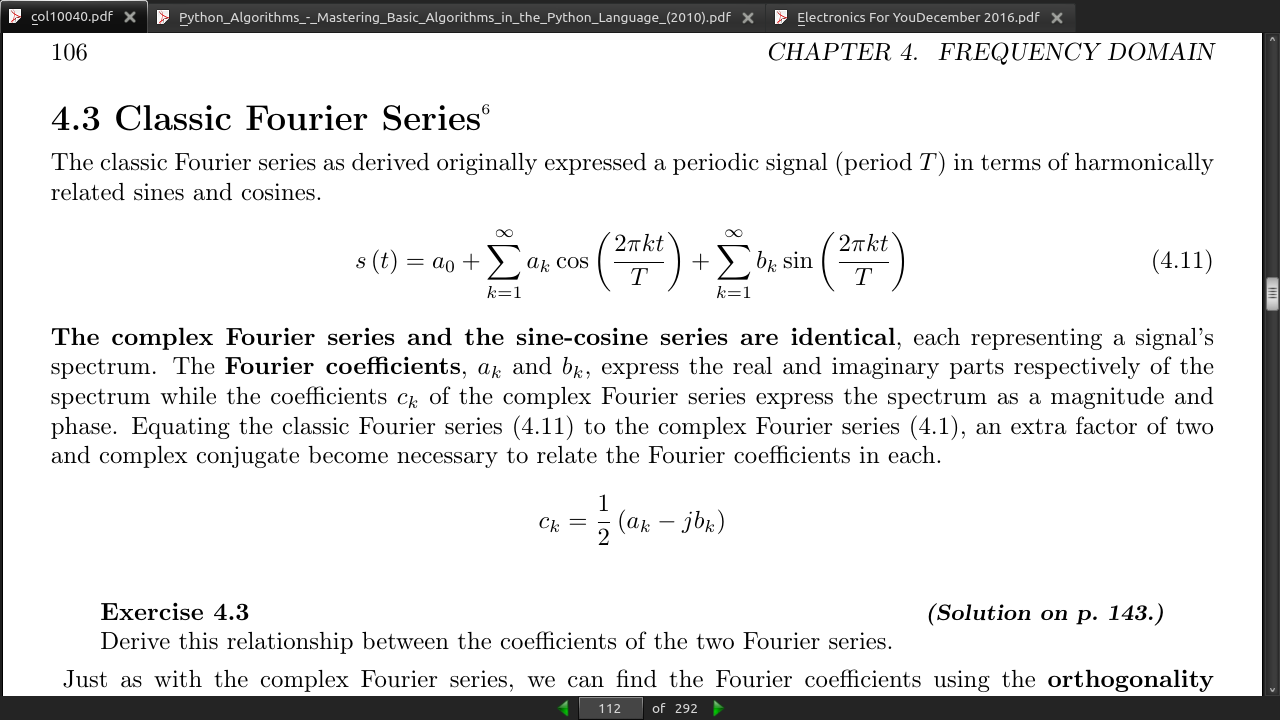
• The complex Fourier series and the sine-cosine series are identical, each representing a signal’s spectrum. The Fourier coefficients, a_k and b_k, express the real and imaginary parts respectively of the spectrum while the coefficients c_k of the complex Fourier series express the spectrum as a magnitude and phase.

• Equating the classic Fourier series (4.11) to the complex Fourier series (4.1), an extra factor of two and complex conjugate become necessary to relate the Fourier coefficients in each.

IMAGE EQ after 4.11

page 114:

• You can unambiguously find the spectrum from the signal (decomposition (4.15)) and the signal from the spectrum (composition). Thus, any aspect of the signal can be found from the spectrum and vice versa. A signal’s frequency domain expression is its spectrum. A periodic signal can be defined either in the time domain (as a function) or in the frequency domain (as a spectrum).

page 115:

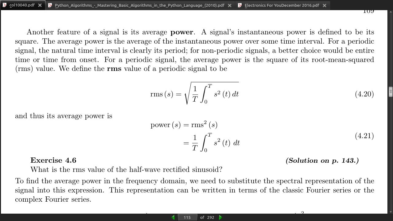
• For a periodic signal, the average power is the square of its root-mean-squared (rms) value. We define the rms value of a periodic signal to be

page 120:

• A new definition of equality is mean-square equality: Two signals are said to be equal in the mean square if rms(s1 − s2) = 0

• The Fourier series value “at” the discontinuity is the average of the values on either side of the jump.

• To encode information we can use the Fourier coefficients.

• Assume we have N letters to encode: {a_1 , …, a_N}. One simple encoding rule could be to make a single Fourier coefficient be non-zero and all others zero for each letter. For example, if an occurs, we make c_n = 1 and c_k = 0, k != n. In this way, the nth harmonic of the frequency 1/T is used to represent a letter. Note N/T that the bandwidth—the range of frequencies required for the encoding—equals . Another possibility is Tto consider the binary representation of the letter’s index. For example, if the letter a_13 occurs, converting 13 to its base-2 representation, we have 13 = 1101. We can use the pattern of zeros and ones to represent directly which Fourier coefficients we “turn on” (set equal to one) and which we “turn off.”

page 122:

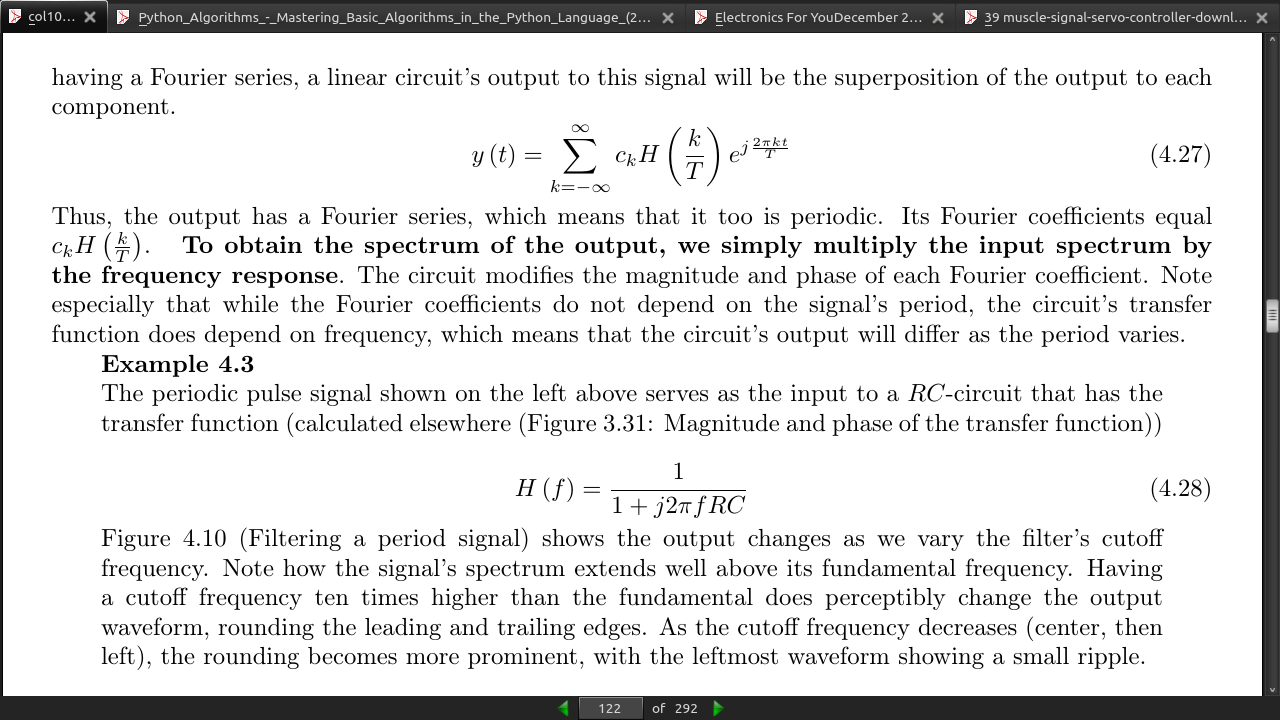
• Because the Fourier series represents a periodic signal as a linear combination of complex exponentials, we can exploit the superposition property. Furthermore, we found for linear circuits that their output to a complex exponential input is just the frequency response evaluated at the signal’s frequency times the complex exponential. Said mathematically, if x(t) = e^(j2πkt)/T, then the output y(t) = H(k/T)*e^(j2πkt)/T because f = k . Thus, if x(t) is periodic thereby having a Fourier series, a linear circuit’s output to this signal will be the superposition of the output to each component.

• Thus, the output has a Fourier series, which means that it too is periodic. Its Fourier coefficients equal c_k*H(k/T). To obtain the spectrum of the output, we simply multiply the input spectrum by Tthe frequency response. The circuit modifies the magnitude and phase of each Fourier coefficient. Note especially that while the Fourier coefficients do not depend on the signal’s period, the circuit’s transfer function does depend on frequency, which means that the circuit’s output will differ as the period varies.

page 123:

• we have calculated the output of a circuit to a periodic input without writing, much less solving, the differential equation governing the circuit’s behavior. Furthermore, we made these calculations entirely in the frequency domain. Using Fourier series, we can calculate how any linear circuit will respond to a periodic input.

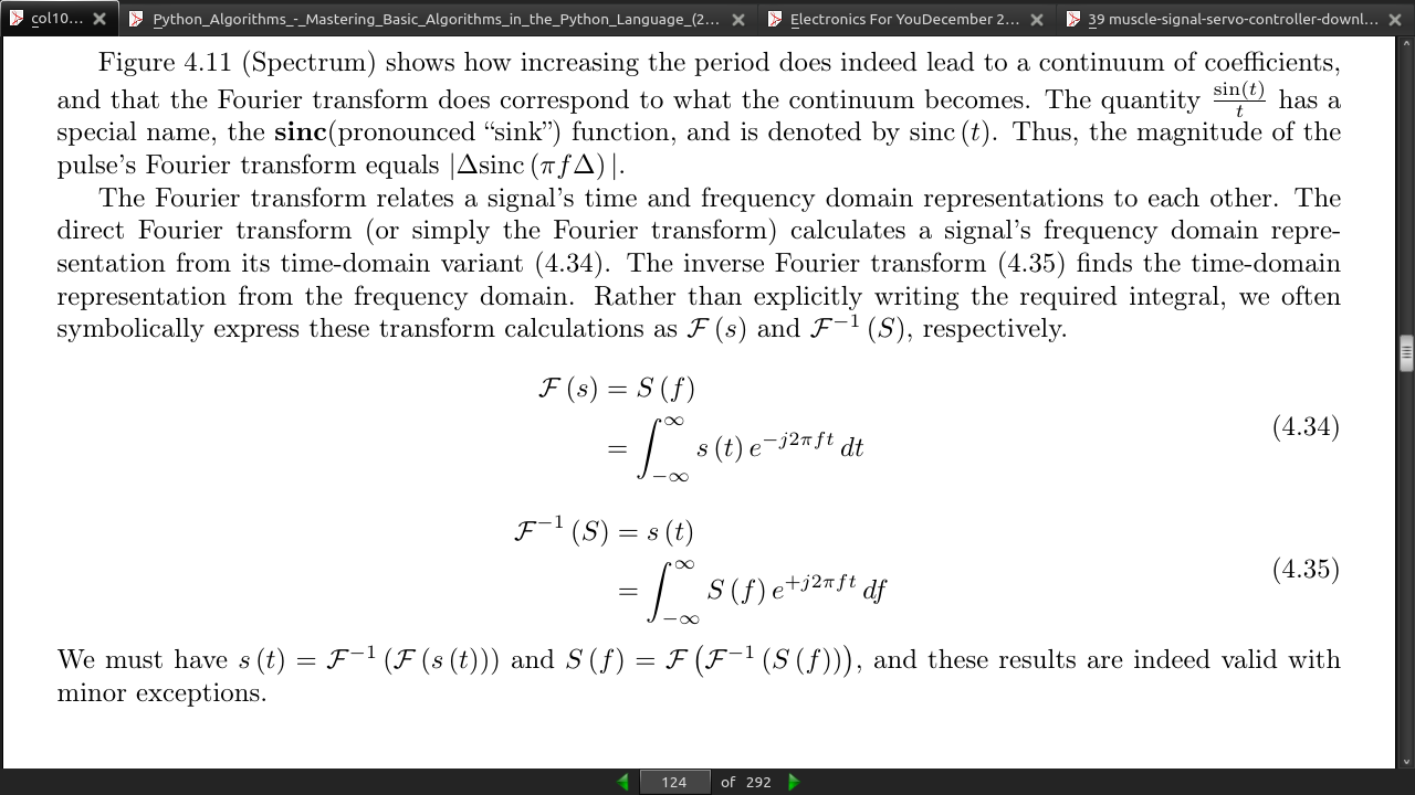
• S(f) is the Fourier transform of s(t) (the Fourier transform is symbolically denoted by the uppercase version of the signal’s symbol) and is defined for any signal for which the integral converges.

page 124:

• The quantity sin(t)/t has a special name, the sinc (pronounced “sink”) function, and is denoted by sinc(t)

• The Fourier transform relates a signal’s time and frequency domain representations to each other. The direct Fourier transform (or simply the Fourier transform) calculates a signal’s frequency domain repre- sentation from its time-domain variant (4.34). The inverse Fourier transform (4.35) finds the time-domain representation from the frequency domain. Rather than explicitly writing the required integral, we often symbolically express these transform calculations as F(s) and F^−1(S), respectively.

page 125:

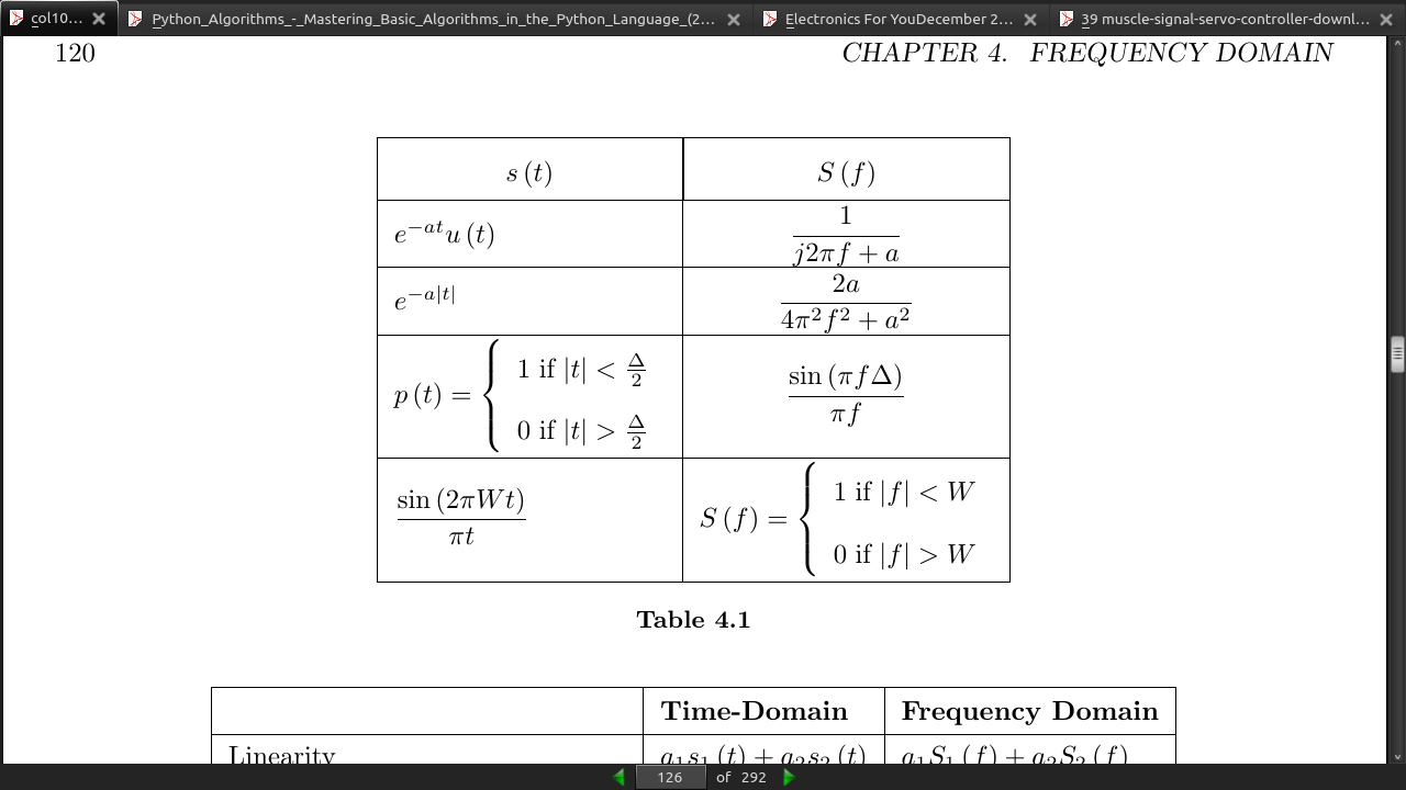
• the mathematical relationships between the time domain and frequency domain versions of the same signal are termed transforms.

• We express Fourier transform pairs as (s(t) <=> S(f)).\

page 129:

• all linear, time-invariant systems have a frequency-domain input-output relation given by the product of the input’s Fourier transform and the system’s transfer function. Thus, linear circuits are a special case of linear, time-invariant systems.

page 130:

• X(f)H1(f) and it serves as the second system’s input, the cascade’s output spectrum is X(f)H1(f)H2(f). Because this product also equals X(f)H2(f)H1(f), the cascade having the linear systems in the opposite order yields the same result. Furthermore, the cascade acts like a single linear system, having transfer function H1(f)H2(f). This result applies to other configurations of linear, time-invariant systems as well;

page 132:

· Chapter 5 - Digital Signal Processing

page 155:

• Note that if we represent truth by a “1” and falsehood by a “0,” binary multiplication corresponds to AND and addition (ignoring carries) to XOR.

page 158:

• Amplitude Quantization = analog signals converted to digital (ADC)

page 159:

• the original amplitude value cannot be recovered without error.

• signal-to-noise ratio, which equals the ratio of the signal power and the quantization error power.

page 161:

page 162:

• each element of the symbolic-valued signal s (n) takes on one of the values {a1, . . . , aK } which comprise the alphabet A.

• 5.6 Discrete-Time Fourier Transform (DTFT)

page 166:

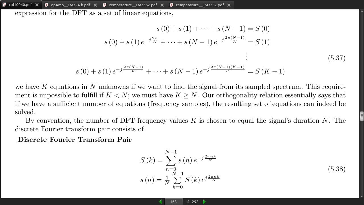
• 5.7 Discrete Fourier Transforms (DFT)

page 168:

page 169:

• 5.9 Fast Fourier Transform (FFT)

• The computational advantage of the FFT comes from recognizing the periodic nature of the discrete Fourier transform. The FFT simply reuses the computations made in the half-length transforms and combines them through additions and the multiplication by e^(−j2πk/N), which is not periodic over N/2, to rewrite the length-N DFT. Figure 5.12 (Length-8 DFT decomposition) illustrates this decomposition.

page 170:

• basic computational element known as a butterfly(Figure 5.13 (Butterfly))

page 171:

• Exervise 5.18 Answer from pg 199: The transform can have any greater than or equal to the actual duration of the signal. We simply “pad” the signal with zero-valued samples until a computationally advantageous signal length results.

page 173:

page 174:

• Exercise 5.22 Answer from page 200: In discrete-time signal processing, an amplifier amounts to a multiplication, a very easy operation to perform.

• linear, shift-invariant systems Slightly different terminology from analog to digital. This is to emphasis integer vals only.

page 175:

• A discrete-time signal s(n) is delayed by n0 samples when we write s(n − n0), with n0 > 0. Choosing n0 to be negative advances the signal along the integers. As opposed to analog delays (Section 2.6.3: Delay), discrete-time delays can only be integer valued. In the frequency domain, delaying a signal corresponds to a linear phase shift of the signal’s discrete-time Fourier transform: s(n − n0) ↔ e^−(j2πfn0)S(e^j2πf)).

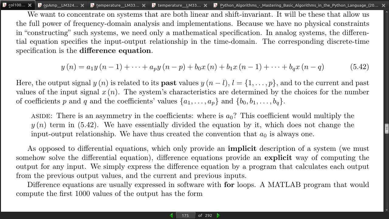
• In analog systems, the differen- tial equation specifies the input-output relationship in the time-domain. The corresponding discrete-time specification is the difference equation.

• Here, the output signal y (n) is related to its past values y (n − l), l = {1, . . . , p}, and to the current and past values of the input signal x (n). The system’s characteristics are determined by the choices for the number of coefficients p and q and the coefficients’ values {a1 , . . . , ap} and {b0, b1 , . . . , bq }.

• Aside: There is an asymmetry in the coefficients: where is a0 ? This coefficient would multiply the y (n) term in (5.42). We have essentially divided the equation by it, which does not change the input-output relationship. We have thus created the convention that a0 is always one.

page 176:

• Set the initial conditions of the difference equation to 0.

page 178:

page 179:

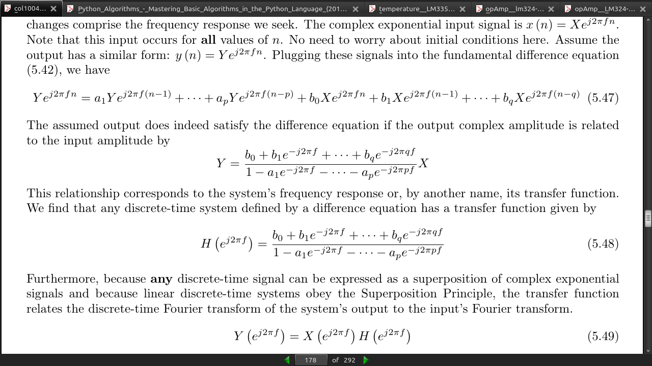
• a unit-sample input, which has X ej2πf = 1, results in the output’s Fourier transform equaling the system’s transfer function.

• In the time-domain, the output for a unit-sample input is known as the system’s unit-sample response, and is denoted by h (n). Combining the frequency-domain and time-domain interpretations of a linear, shift- invariant system’s unit-sample response, we have that h (n) and the transfer function are Fourier transform pairs in terms of the discrete-time Fourier transform.

page 180:

• (sampling in one domain, be it time or frequency, can result in aliasing in the other) unless we sample fast enough. Here, the duration of the unit-sample response determines the minimal sampling rate that prevents aliasing.

• For IIR systems, we cannot use the DFT to find the system’s unit-sample response: aliasing of the unit- sample response will always occur. Consequently, we can only implement an IIR filter accurately in the time domain with the system’s difference equation. Frequency-domain implementations are restricted to FIR filters.

page 181:

• The spectrum resulting from the discrete-time Fourier transform depends on the continuous frequency variable f . That’s fine for analytic calculation, but computationally we would have to make an uncountably infinite number of computations.

page 185:

• we can process, in particular filter, analog signals “with a computer” by constructing the system shown in Figure 5.24. To use this system, we are assuming that the input signal has a lowpass spectrum and can be bandlimited without affecting important signal aspects. Bandpass signals can also be filtered digitally, but require a more complicated system. Highpass signals cannot be filtered digitally.

page 186:

• It could well be that in some problems the time-domain version is more efficient (more easily satisfies the real time requirement), while in others the frequency domain approach is faster. In the latter situations, it is the FFT algorithm for computing the Fourier transforms that enables the superiority of frequency-domain implementations.

· Chapter 6 - Information Communication

page 202:

• In the case of single-wire communications, the earth is used as the current’s return path. In fact, the term ground for the reference node in circuits originated in single-wire telegraphs.

page 203:

page 207:

• Transmitted signal amplitude does decay exponentially along the transmission line. Note that in the high-frequency regime the space constant is small, which means the signal attenuates little.

• Wireless channels exploit the prediction made by Maxwell’s equation that electromagnetic fields propagate in free space like light. When a voltage is applied to an antenna, it creates an electromagnetic field that propagates in all directions (although antenna geometry affects how much power flows in any given direction) that induces electric currents in the receiver’s antenna.

• The fundamental equation relating frequency and wavelength for a propagating wave is

• Thus, wavelength and frequency are inversely related: High frequency corresponds to small wavelengths. For example, a 1 MHz electromagnetic field has a wavelength of 300 m. Antennas having a size or distance from the ground comparable to the wavelength radiate fields most efficiently. Consequently, the lower the frequency the bigger the antenna must be. Because most information signals are baseband signals, having spectral energy at low frequencies, they must be modulated to higher frequencies to be transmitted over wireless channels.

page 208:

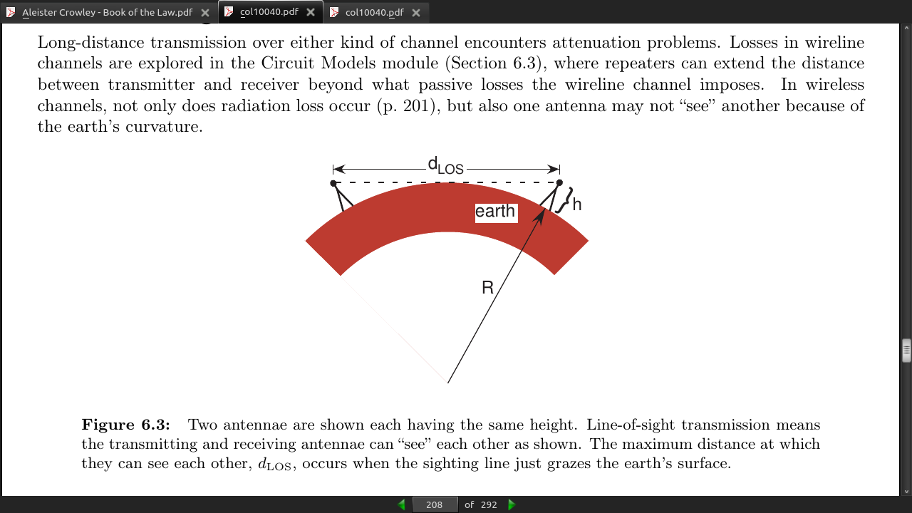
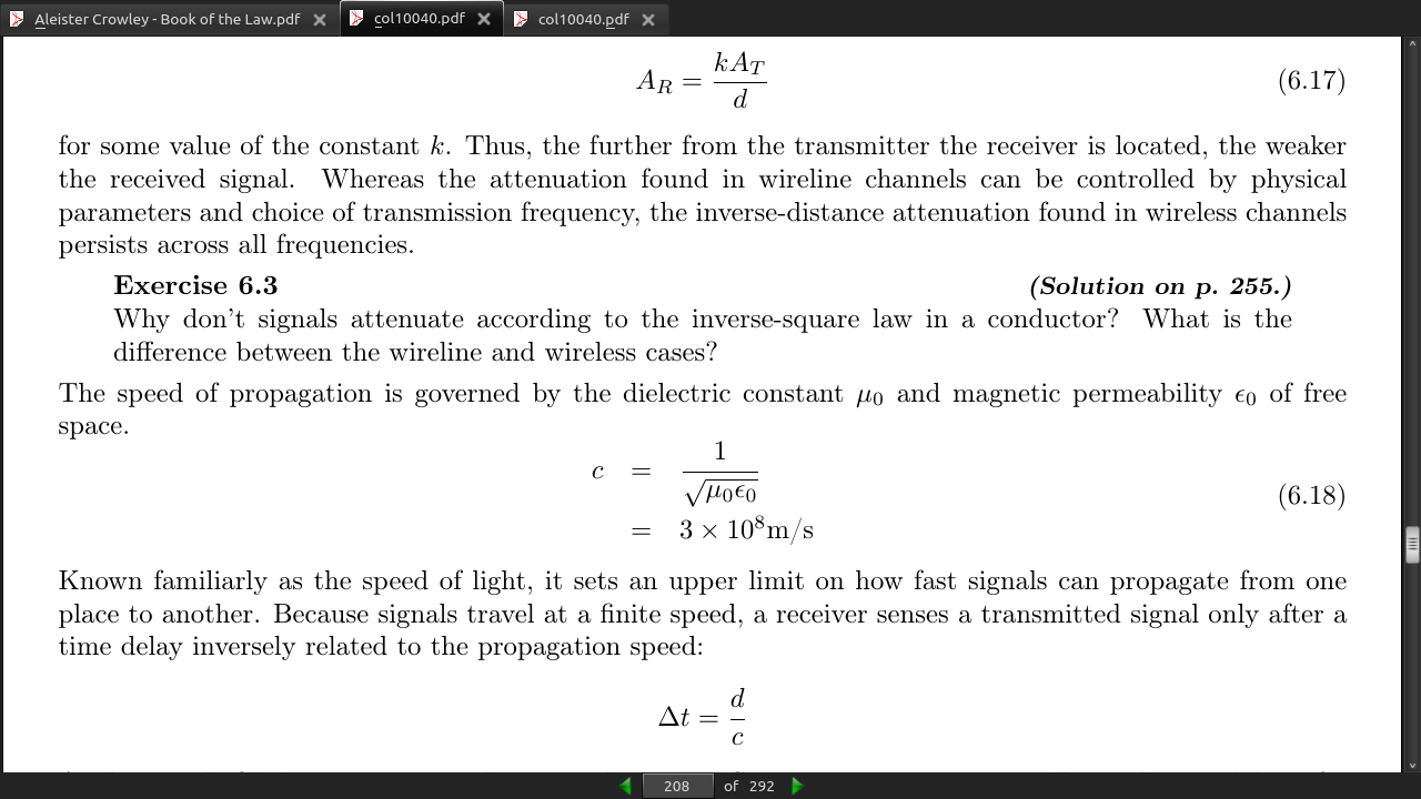
• At the speed of light, a signal travels across the United States in 16 ms, a reasonably small time delay. If a lossless (zero space constant) coaxial cable connected the East and West coasts, this delay would be two to three times longer because of the slower propagation speed.

page 209:

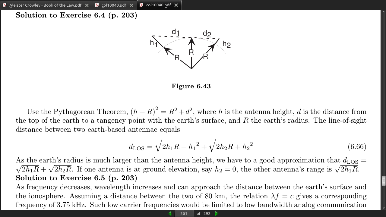
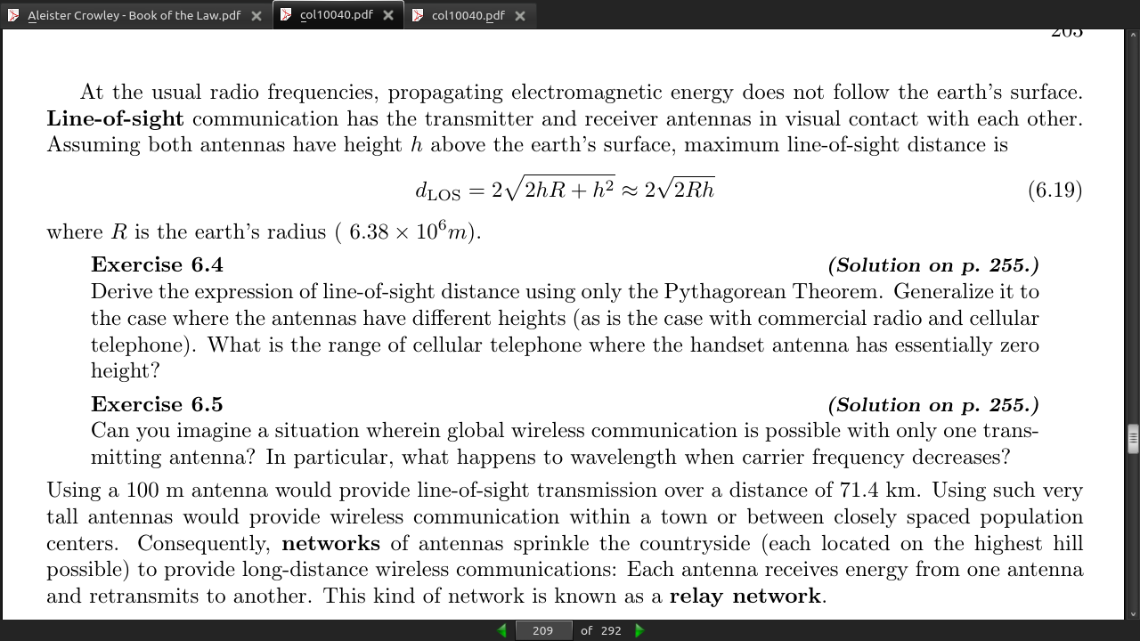
• The maximum distance along the earth’s surface that can be reached by a single ionospheric reflection is 2Rarccos(R/R+h_i), which ranges between 2,010 and 3,000 km when we substitute minimum and maximum ionospheric altitudes (80-180km).

• delays of 6.8-10ms for a single reflection.

page 210:

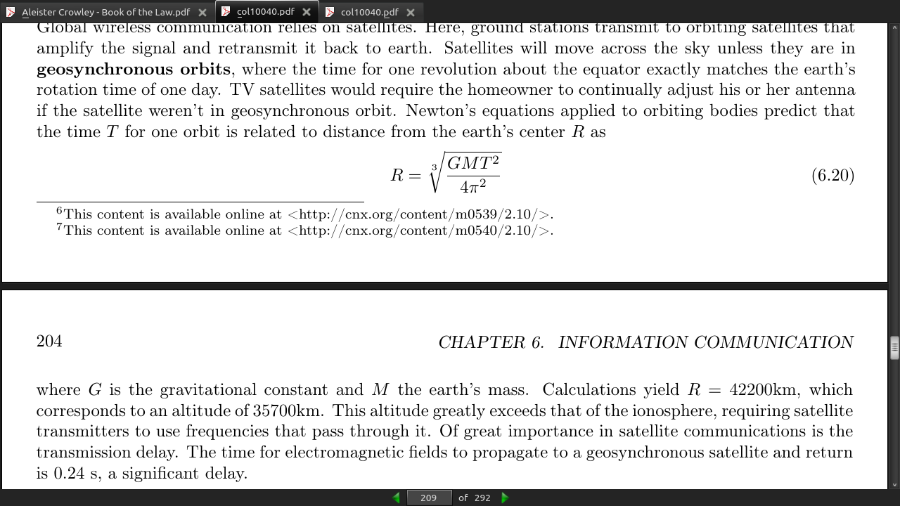
• geosynchronous satallites need to be at at altitude of 35700km. They also need to work on frequencies not blocked by the ionosphere. Their delay si about 0.24 seconds.

page 211:

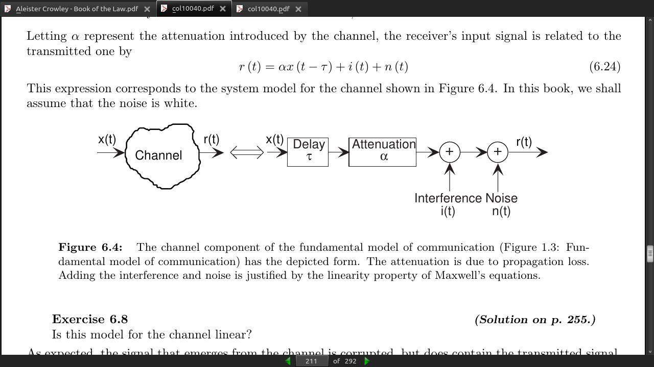
page 216:

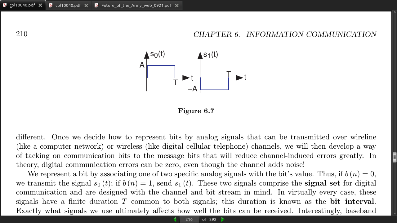
• A commonly used example of a signal set consists of pulses that are negatives of each other (Figure 6.7).

s0(t) = ApT(t) s1(t) = −ApT(t)

• This way of representing a bit stream—changing the bit changes the sign of the transmitted signal—is known as binary phase shift keying and abbreviated BPSK.

• The datarate R of a digital communication system is how frequently an information bit is transmitted. In this example it equals the reciprocal of the bit interval: R = 1/T. Thus, for a 1 Mbps (megabit per second) transmission, we must have T = 1μs.

page 217:

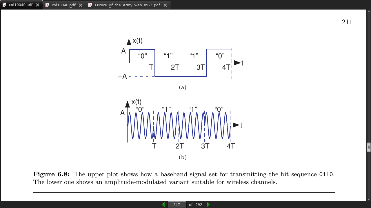
page 218:

• The first and third harmonics contain that fraction of the total power, meaning that the effective bandwidth of our baseband signal is 3/2T or, expressing this quantity in terms of the datarate, 3R/2. Thus, a digital communications signal requires more bandwidth than the datarate: a 1 Mbps baseband system requires a bandwidth of at least 1.5MHz. Listen carefully when someone describes the transmission bandwidth of digital communication systems: Did they say “megabits” or “megahertz?”

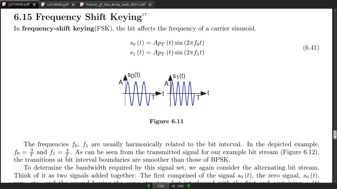
• In frequency-shift keying(FSK), the bit affects the frequency of a carrier sinusoid.

page 219:

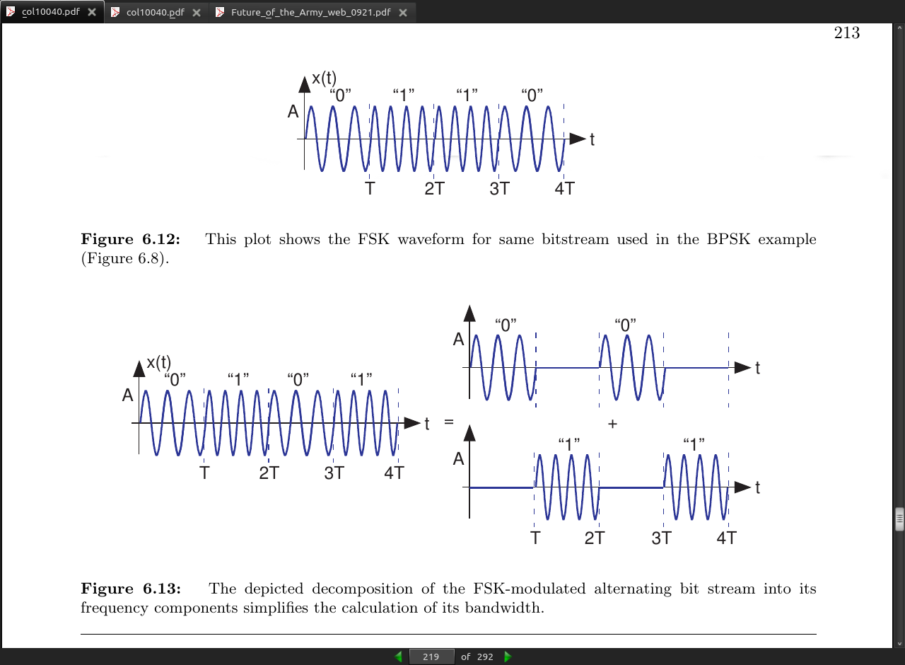
• Synchronization can occur because the transmitter begins sending with a reference bit sequence, known as the preamble. This reference bit sequence is usually the alternating sequence as shown in the square wave example19 and in the FSK example (Figure 6.13).

• This procedure amounts to what in digital hardware as self-clocking signaling:

page 220:

• The second preamble phase informs the receiver that data bits are about to come and that the preamble is almost over.

page 222:

page 230:

page 223:

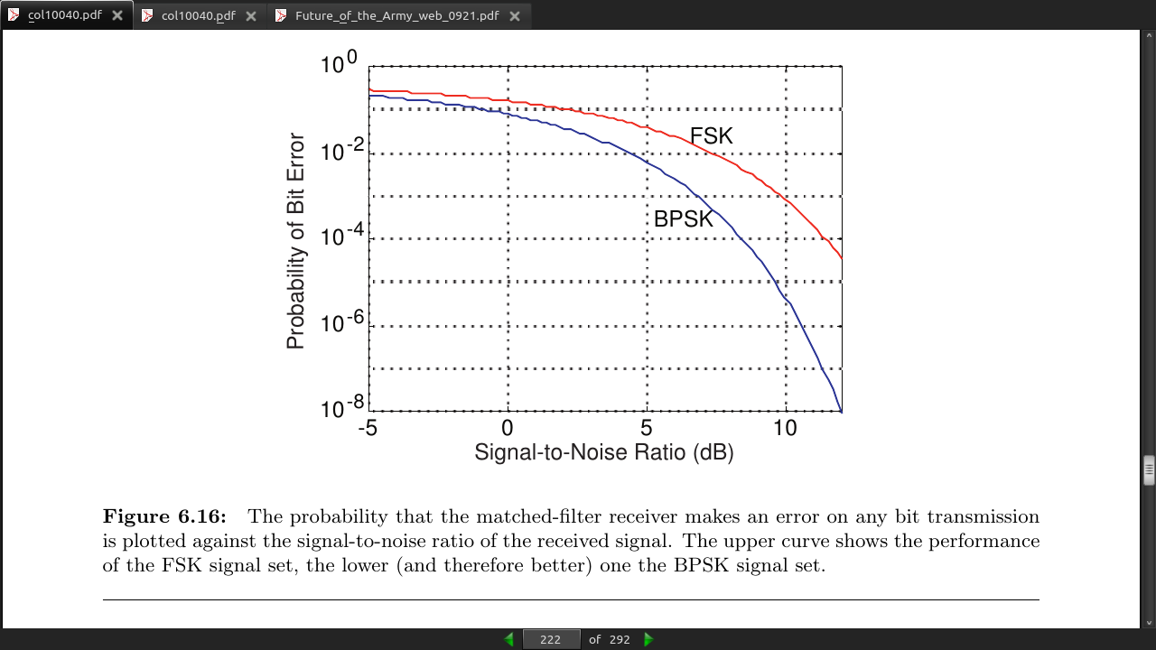
• As the received signal becomes increasingly noisy, whether due to increased distance from the transmit- ter (smaller α) or to increased noise in the channel (larger N_0), the probability the receiver makes an error approaches 1/2.

• As the signal-to-noise ratio increases, performance gains–smaller probability of error pe – can be easily obtained. At a signal-to-noise ratio of 12 dB, the probability the receiver makes an error equals 10−8. In words, one out of one hundred million bits will, on the average, be in error.

• Once the signal-to-noise ratio exceeds about 5 dB, the error probability decreases dramatically. Adding 1 dB improvement in signal-to-noise ratio can result in a factor of ten smaller pe .

page 224:

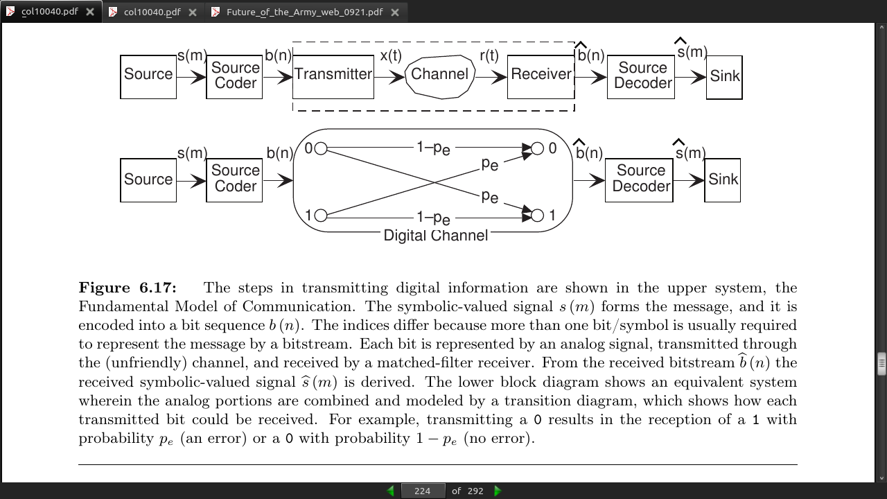
page 226:

• Shannon’s Source Coding Theorem (6.52) has additional applications in data compression.

• Lossy and lossless

page 227:

1. Create a vertical table for the symbols, the best ordering being in decreasing order of probability.

2. Form a binary tree to the right of the table. A binary tree always has two branches at each node. Build the tree by merging the two lowest probability symbols at each level, making the probability of the node equal to the sum of the merged nodes’ probabilities. If more than two nodes/symbols share the lowest probability at a given level, pick any two; your choice won’t affect B (A).

3. At each node, label each of the emanating branches with a binary number. The bit sequence obtained from passing from the tree’s root to the symbol is its Huffman code.

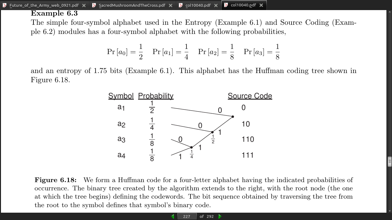
page 228:

• Huffman showed that his (maximally efficient) code had the prefix property: No code for a symbol began another symbol’s code. Once you have the prefix property, the bitstream is partially self-synchronizing: Once the receiver knows where the bitstream starts, we can assign a unique and correct symbol sequence to the bitstream.

• Otherwise you need a “comma” or some seperator but between each symbol.

page 229:

• Telegraph deployed in 1844!

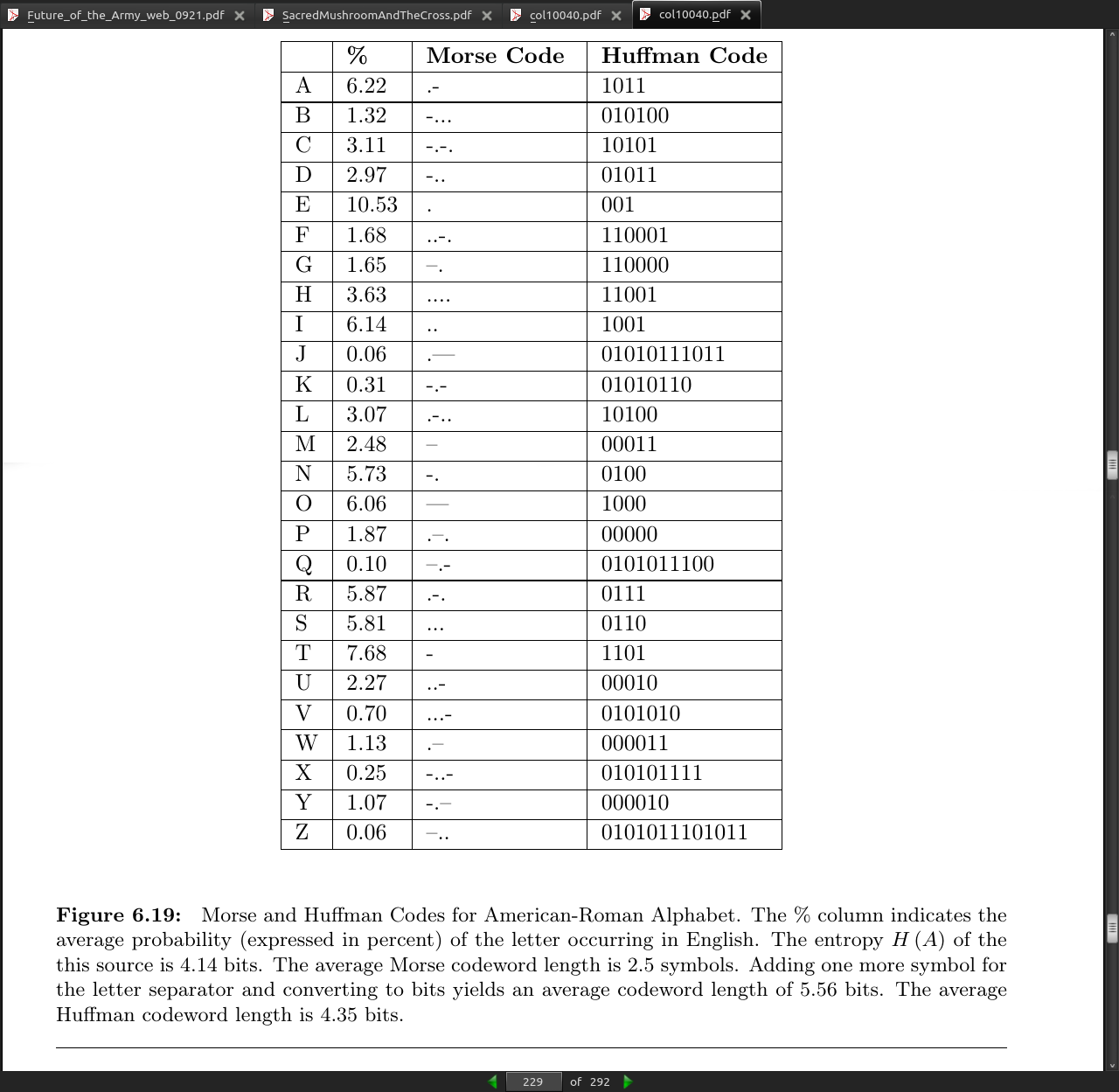
page 230:

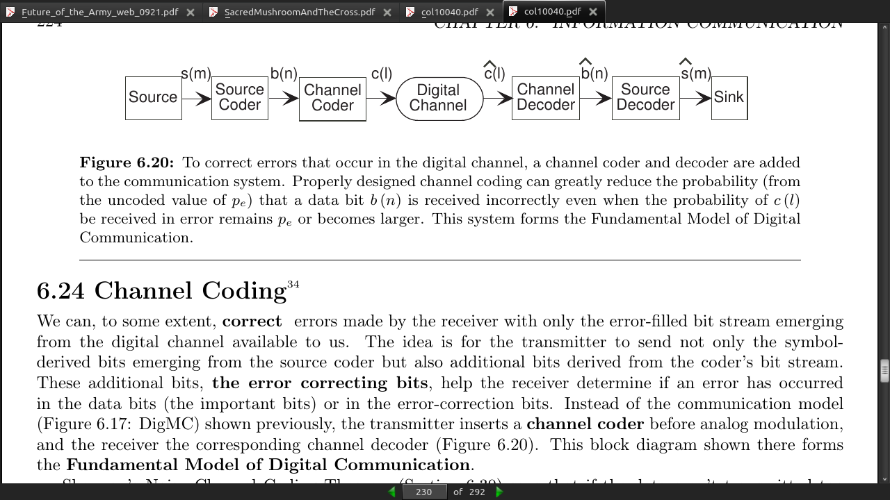
• Adding a channel coder and decoder to each end of the digital channel allows for error correcting bits to reduce errors further. This is the Fundamental Model of Digital Communication.

FIG 6.20

• Repetition code sends an odd number of bits (repeated) and then votes to see what the value is. The repeated code has a higher datarate which makes the scheme inefficient. Transmitting 3 bits for every 1 does not make up in accuracy what you lose in speed.

page 233:

• We define the Hamming distance between binary data words c1 and c2 , denoted by d(c1,c2) to be the minimum number of bits that must be “flipped” to go from one word to the other.

page 242:

• Communications networks are now categorized according to whether they use packets or not. A system like the telephone network is said to be circuit switched: The network establishes a fixed route that lasts the entire duration of the message. Circuit switching has the advantage that once the route is determined, the users can use the capacity provided them however they like. Its main disadvantage is that the users may not use their capacity efficiently, clogging network links and nodes along the way. Packet-switched networks continuously monitor network utilization, and route messages accordingly. Thus, messages can, on the average, be delivered efficiently, but the network cannot guarantee a specific amount of capacity to the users.

page 246:

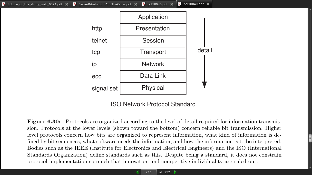
· Appendix

page 270:

• FCC Frequency Allocation chart