Home · Book Reports · 2017 · Python Algorithms - Mastering Basic Algorithms in the Python Language

- Author :: Magnus Lie Hetland
- Publication Year :: 2010
- Read Date :: 2017-03-22
- Source :: Python_Algorithms_-_Mastering_Basic_Algorithms_in_the_Python_Language_(2010).pdf
designates my notes. / designates important.
Thoughts
Not for beginners, but if you have a programming language (not python per se as python is pretty close to pseudo) under your belt and aren’t afraid of equations containing funny Greek squiggles, this can provide a lot of insight into problem solving in general.
Graphs are certainly not anything close to new, but with the advent of social media they have come into the “mainstream”. Even so, the graphs discussed here don’t have much in common with the typical social network. They are used here to solve problems that are (sometimes) not intuitively seen as graph problems.
It includes a LOT of code snippets that are well commented as well as list (in the appendixes) of common algorithms and problems. It seems like it might be a worthy reference if you are looking for an algorithmic solution, but aren’t sure which one you need. Heck, you might not even be sure what you problem is and how it might be able to be tweaked so as to take advantage of a time-tested solution.
Table of Contents
- Chapter 01: Introduction
- Chapter 02: The Basics
- Chapter 03: Counting 101
- Chapter 04: Induction and Recursion... and Reduction
- Chapter 05: Traversal: The Skeleton Key of Algorithmics
- Chapter 06: Divide, Combine, and Conquer
- Chapter 07: Greed Is Good? Prove It!
- Chapter 08: Tangled Dependencies and Memoization
- Chapter 09: From A to B with Edsger and Friends
- Chapter 10: Matchings, Cuts, and Flows
- Chapter 11: Hard Problems and (Limited) Sloppiness
· Chapter 1: Introduction
page 7:
- Cormen, T. H., Leiserson, C. E., Rivest, R. L., and Stein, C. (2009). Introduction to Algorithms, second edition. MIT Press.
· Chapter 2: The Basics
page 13:
-
The expression O(g), for some function g(n), represents a set of functions, and a function f (n) is in this set if it satisfies the following condition: there exists a natural number n0 and a positive constant c such that f (n) ≤ cg(n) for all n ≥ n0.
-
In other words, if we’re allowed to tweak the constant c (for example, by running the algorithms on machines of different speeds), the function g will eventually (that is, at n0) grow bigger than f. See Figure 2-1 for an example.
-
omega, the opposite of big oh: f(n) ≥ cg(n)

page 14:
-
Note Our first two asymptotic operators, O and Ω, are each others’ inverses: if f is O(g ), then g is Ω(f ).
-
The sets formed by Θ are simply intersections of the other two, that is, Θ(g) = O(g) ∩ Ω(g).
page 15:
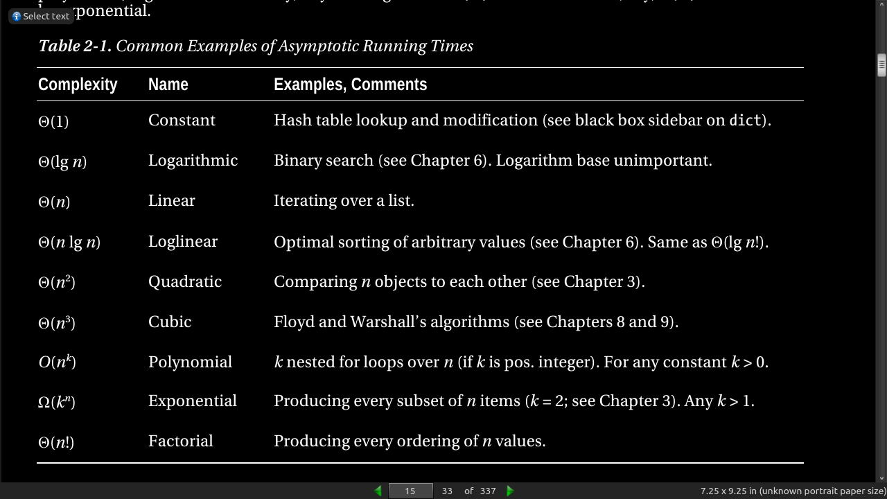
page 16:
-
In a sum, only the dominating summand matters. For example, Θ(n2 + n3 + 42) = Θ(n3).
-
In a product, constant factors don’t matter. For example, Θ(4.2n lg n) = Θ(n lg n).
page 20:
- If you have a tweak you think will improve your program, try it! Implement the tweak, and run some experiments. Is there an improvement? And if the tweak makes your code less readable and the improvement is small, is it really worth it?
page 21:
-
Tip 2: For timing things, use timeit. (module)
-
If you want to time a function (which could, for example, be a test function wrapping parts of your code), it may be even easier to use timeit from the shell command line, using the -m switch: $ python -m timeit -s"import mymodule as m" “m.myfunction()”
import cProfile
cProfile.run('main()')
- want to empirically examine the behavior of your algorithm on a given problem instance, the trace module in the standard library can be useful
page 23:
-
In many cases, if you can formulate what you’re working on as a graph problem, you’re (at least) halfway to a solution. And if your problem instances are in some form expressible as trees, you stand a good chance of having a really efficient solution.
-
Trees are just a special kind of graphs, so most algorithms and representations for graphs will work for them as well.
page 25:
- What this means to us is that accessing elements of a dict or set can be assumed to take constant (expected) time, which makes them highly useful building blocks for more complex structures and algorithms.
page 26:
- Listing 2-1. A Straightforward Adjacency Set Representation:
a, b, c, d, e, f, g, h = range(8)
N = [
{b, c, d, e, f}, # a
{c, e}, # b
{d}, # c
{e}, # d
{f}, # e
{c, g, h}, # f
{f, h}, # g
{f, g}  # h
]
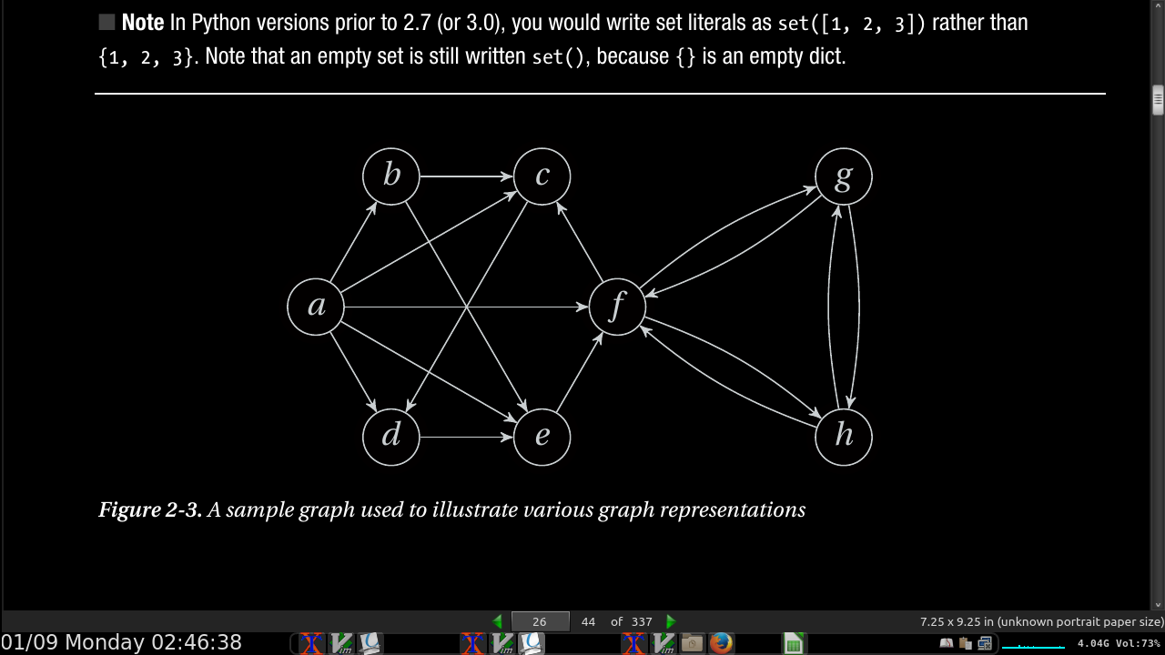
page 27:
- in our code, N[v] is now a set of v’s neighbors. Assuming you have defined N as earlier in an interactive interpreter, you can now play around with the graph:
>>> b in N[a] # Neighborhood membership
True
>>> len(N[f]) # Degree
3
- Can use lists over sets, is slower but has less overhead if all you have is smaller data sets.
page 28:
-
Yet another minor tweak on this idea is to use dicts instead of sets or lists. The neighbors would then be keys in this dict, and you’d be free to associate each neighbor (or out-edge) with some extra value, such as an edge weight. How this might look is shown in Listing 2-3 (with arbitrary edge weights added).
-
Listing 2-3. Adjacency dicts with Edge Weights:
a, b, c, d, e, f, g, h = range(8)
N = [
{b:2, c:1, d:3, e:9, f:4}, # a
{c:4, e:3}, # b
{d:8}, # c
{e:7}, # d
{f:5}, # e
{c:2, g:2, h:2}, # f
{f:1, h:6}, # g
{f:9, g:8} # h
]
- The adjacency dict version can be used just like the others, with the additional edge weight functionality:
>>> b in N[a] # Neighborhood membership
True
>>> len(N[f]) # Degree
3
>>> N[a][b]
 # Edge weight for (a, b)
2
page 29:
- Listing 2-4. A Dict with Adjacency Sets:
N = {
'a': set('bcdef'),
'b': set('ce'),
'c': set('d'),
'd': set('e'),
'e': set('f'),
'f': set('cgh'),
'g': set('fh'),
'h': set('fg')
}
- This, a dictionary with adjacency lists, is what Guido van Rossum uses in his article “Python Patterns— Implementing Graphs,” which is found online at http://www.python.org/doc/essays/graphs.html
page 30:
- inf or float(inf) == infinity
page 34:
class Bunch(dict):
def __init__(self, *args, **kwds):
super(Bunch, self).__init__(*args, **kwds)
self.__dict__ = self
- There are several useful aspects to this pattern. First, it lets you create and set arbitrary attributes by supplying them as command-line arguments:
>>> x = Bunch(name="Jayne Cobb", position="Public Relations")
>>> x.name
'Jayne Cobb'
Second, by subclassing dict, you get lots of functionality for free, such as iterating over the keys/attributes
or easily checking whether an attribute is present. Here’s an example:
>>> T = Bunch
>>> t = T(left=T(left="a", right="b"), right=T(left="c"))
>>> t.left
{'right': 'b', 'left': 'a'}
>>> t.left.right
'b'
>>> t['left']['right']
'b'
>>> "left" in t.right
True
>>> "right" in t.right
False
page 37:
-
if your program is fast enough, there’s no need to optimize it.
-
If you are doing multiple lookups in a list, it may be faster to cast it as a set.
-
(without the optimizations) you need to create a new string for every += operation,
>>> s = ""
>>> for chunk in input():
... s += chunk
- A better solution would be the following:
>>> chunks = []
>>> for chunk in input():
... chunks.append(chunk)
...
>>> s = ''.join(chunks)
- You could even simplify this further:
>>> s = ''.join(input())
page 38:
- Quadratic
>>> result = sum(lists, [])
- Faster
>>> res = []
>>> for lst in lists:
... res.extend(lst)
page 39:
- Float inaccuracy:
>>> sum(0.1 for i in range(10)) == 1.0
False
-
never compare floats for equality.
-
check whether they are approximately equal. For example, you could take the approach of assertAlmostEqual from the unittest module:
>>> def almost_equal(x, y, places=7):
... return round(abs(x-y), places) == 0
...
>>> almost_equal(sum(0.1 for i in range(10)), 1.0)
True
- There are also tools you can use if you need exact decimal floating-point numbers, for example the decimal module:
>>> from decimal import *
>>> sum(Decimal("0.1") for i in range(10)) == Decimal("1.0")
True
- sage calculates exact values, sagemath.org, but sage is much slower.
· Chapter 3: Counting 101
page 46:
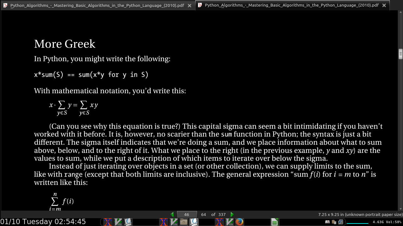

page 47:
- a technical meaning of the word tournament in graph theory (a complete graph, where each edge is assigned a direction
page 48:
- round-robin events are = n(n –1)/2, where n is the number of participants.
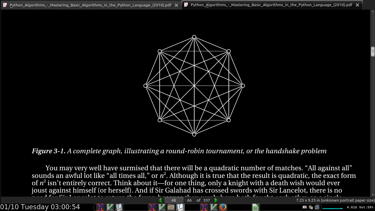
page 49:
-
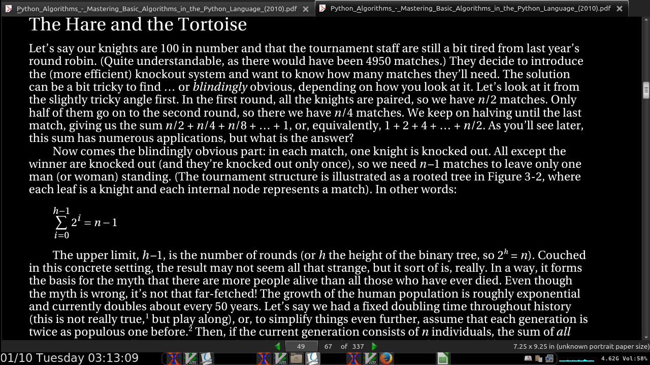
In a single elimination/knockout tournament:
-
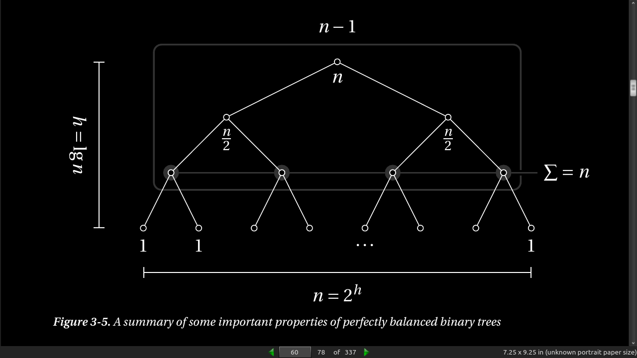
In the first round, all the knights are paired, so we have n/2 matches. Only half of them go on to the second round, so there we have n/4 matches. We keep on halving until the last match, giving us the sum n/2 + n/4 + n/8 + … + 1, or, equivalently, 1 + 2 + 4 + … + n/2.
-
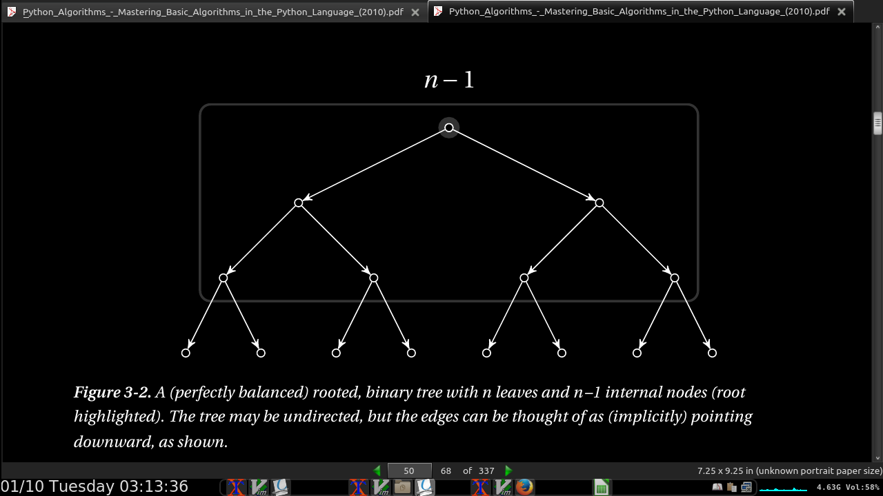
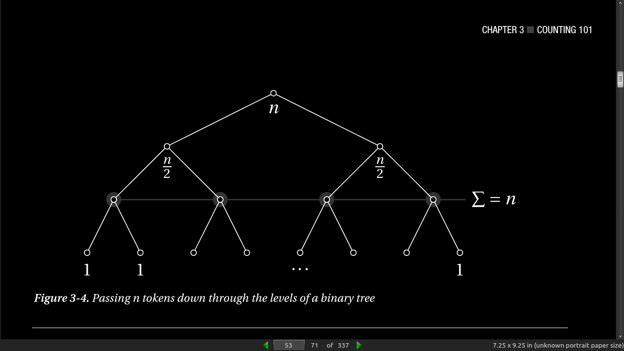
The upper limit, h –1, is the number of rounds (or h the height of the binary tree, so 2^h = n).
page 50:
- summing up the powers of two, you always get one less than the next power of two. For example, 1 + 2 + 4 = 8 – 1, or 1 + 2 + 4 + 8 = 16 – 1, and so forth.
page 51:
- Binary searching, how to solve how many “cuts” is needed with log base 2
>>> from random import randrange
>>> n = 10**90
>>> p = randrange(10**90)

>>> p < n/2 #cut the search in half
True

>>> from math import log
>>> log(n, 2) # base-two logarithm
298.97352853986263 #how many guesses to always win

page 53:
page 54:
- Permutations are calculated with factorial.

- Combinations are calculated with binomial coefficients. C(n,k) or “n choose k”
page 56:
- Recursion and Recurrences
page 58:
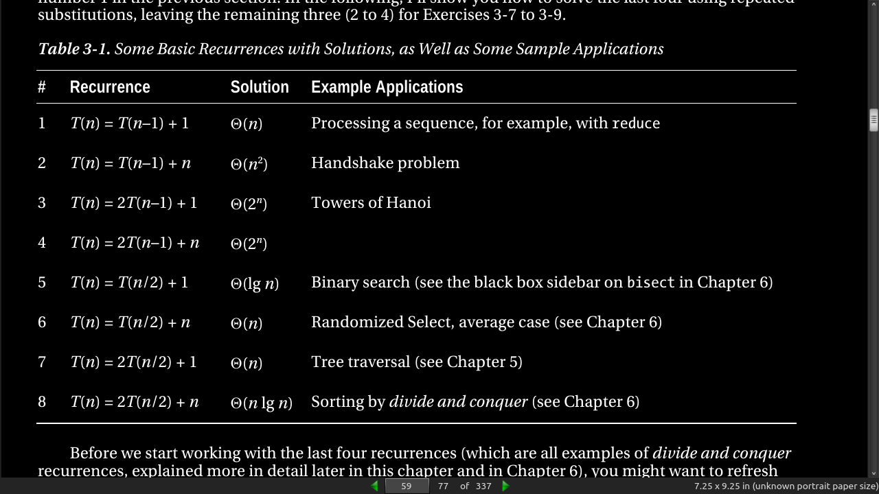
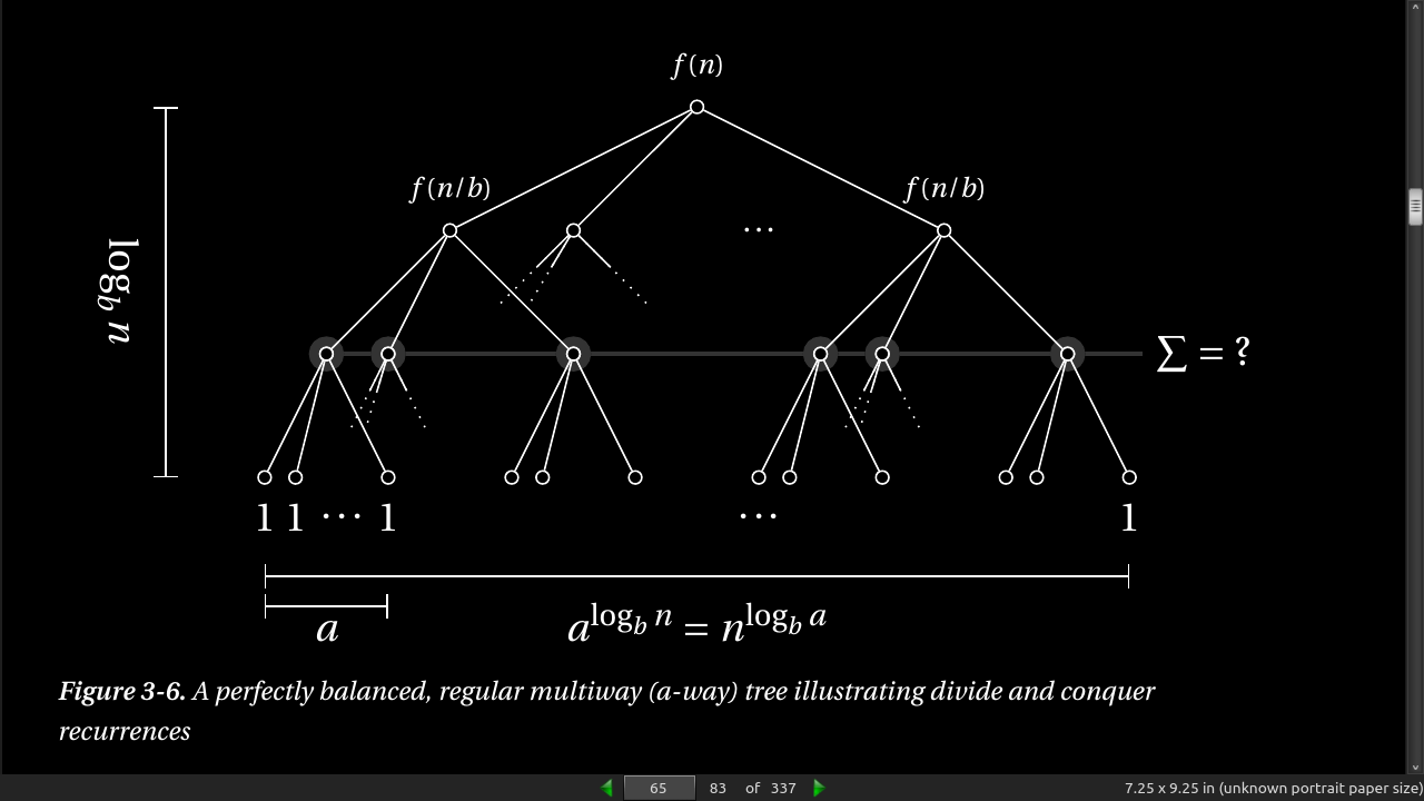
- The general form of the recurrences you’ll normally encounter is is T(n) = a * T(g(n)) + f(n), where a represents the number of recursive calls, g(n) is the size of each subproblem to be solved recursively, and f(n) is any extra work done in the function, in addition to the recursive calls.
page 59:
page 60:
page 65:
· Chapter 4: Induction and Recursion… and Reduction
page 71:
-
Reduction means transforming one problem to another. We normally reduce an unknown problem to one we know how to solve. The reduction may involve transforming both the input (so it works with the new problem) and the output (so it’s valid for the original problem).
-
Induction (or, mathematical induction) is used to show that a statement is true for a large class of objects (often the natural numbers). We do this by first showing it to be true for a base case (such as the number 1) and then showing that it “carries over” from one object to the next (if it’s true for n –1, then it’s true for n).
-
Recursion is what happens when a function calls itself. Here we need to make sure the function works correctly for a (nonrecursive) base case and that it combines results from the recursive calls into a valid solution.
page 78:
- There is usually less overhead with using a loop than with recursion (so it can be faster), and in most languages (Python included), there is a limit to how deep the recursion can go (the maximum stack depth).
page 79:
'''Listing 4-1. Recursive Insertion Sort'''
def ins_sort_rec(seq, i):
  if i==0: return                        #Base case -- do nothing
  ins_sort_rec(seq, i-1)                 #Sort 0..i-1
  j = i                                  #Start "walking" down
  while j > 0 and seq[j-1] > seq[j]:     #Look for OK spot
  seq[j-1], seq[j] = seq[j], seq[j-1]    #Keep moving seq[j] down
  j -= 1                                 #Decrement j
'''Listing 4-2. Insertion Sort'''
def ins_sort(seq):
  for i in range(1,len(seq)):             #0..i-1 sorted so far
    j = i                                 #Start "walking" down
    while j > 0 and seq[j-1] > seq[j]:    #Look for OK spot
      seq[j-1], seq[j] = seq[j], seq[j-1] #Keep moving seq[j] down
      j -= 1                              #Decrement j
- 7 These algorithms aren’t all that useful, but they’re commonly taught, because they serve as excellent examples. Also, they’re classics, so any algorist should know how they work.
page 80:
-
Listing 4-3. Recursive Selection Sort
-
Listing 4-4. Selection Sort
-
The recursive implementation explicitly represents the inductive hypothesis (as a recursive call), while the iterative version explicitly represents repeatedly performing the inductive step.
-
These are two major variations of reductions: reducing to a different problem and reducing to a shrunken version of the same. If you think of the subproblems as vertices and the reductions as edges, you get the subproblem graph discussed in Chapter 2, a concept I’ll revisit several times. (It’s especially important in Chapter 8.)
page 81:
page 82:
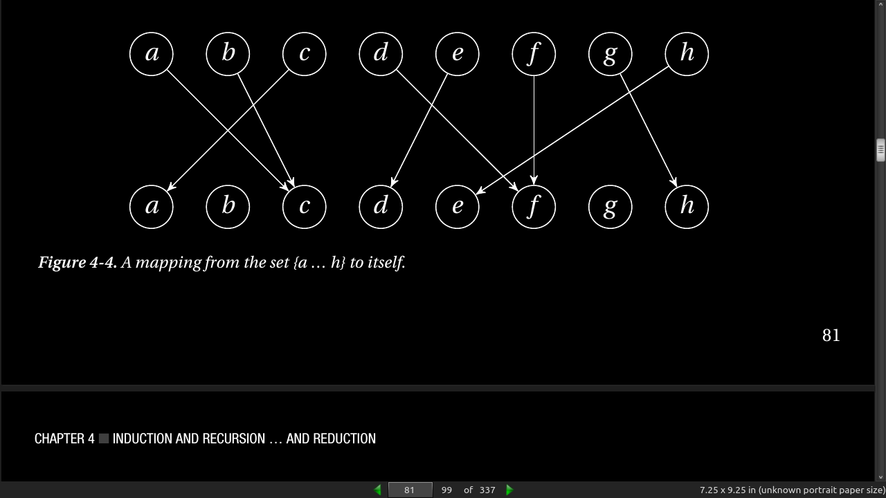
- in essence, a mapping like this is just a position (0…n –1) associated with each element (also 0…n –1), and we can implement this using a simple list. For example, the example in Figure 4-4 (if a = 0, b = 1, …) can be represented as follows:
>>> M = [2, 2, 0, 5, 3, 5, 7, 4]
>>>
0
- Tip When possible, try to use a representation that is as specific to your problem as possible. More general representations can lead to more bookkeeping and complicated code; if you use a representation that implicitly embodies some of the constraints of the problem, both finding and implementing a solution can be much easier.
page 83:
'''Listing 4-5. A Naïve Implementation of the Recursive Algorithm Idea
   for Finding a Maximum Permutation'''
def naive_max_perm(M, A=None):
  if A is None:                   # The elt. set not supplied?
    A = set(range(len(M)))        # A = {0, 1, ... , n-1}
  if len(A) == 1: return A        # Base case -- single-elt. A
  B = set(M[i] for i in A)        # The "pointed to" elements
  C = A - B                       # "Not pointed to" elements
  if C:                           # Any useless elements?
    A.remove(C.pop())             # Remove one of them
    return naive_max_perm(M, A)   # Solve remaining problem
  return A                        # All useful -- return all

>>> naive_max_perm(M)
{0, 2, 5} # So, a, c, and f can take part in the permutation.
page 84:
- Tip In recent versions of Python, the collections module contains the Counter class, which can count (hashable) objects for you.
page 85:
from collections import defaultdict

def counting_sort(A, key=lambda x: x):
  B, C = [], defaultdict(list)       # Output and "counts"
  for x in A:
    C[key(x)].append(x)              # "Count" key(x)
  for k in range(min(C), max(C)+1):  # For every key in the range
    B.extend(C[k])                   # Add values in sorted order
  return B
-
By default, I’m just sorting objects based on their values. By supplying a key function, you can sort by anything you’d like.
-
key() in C[].append() is interesting.
page 87:
-
the tasks to be undertaken will have dependencies that partially restrict their ordering.
-
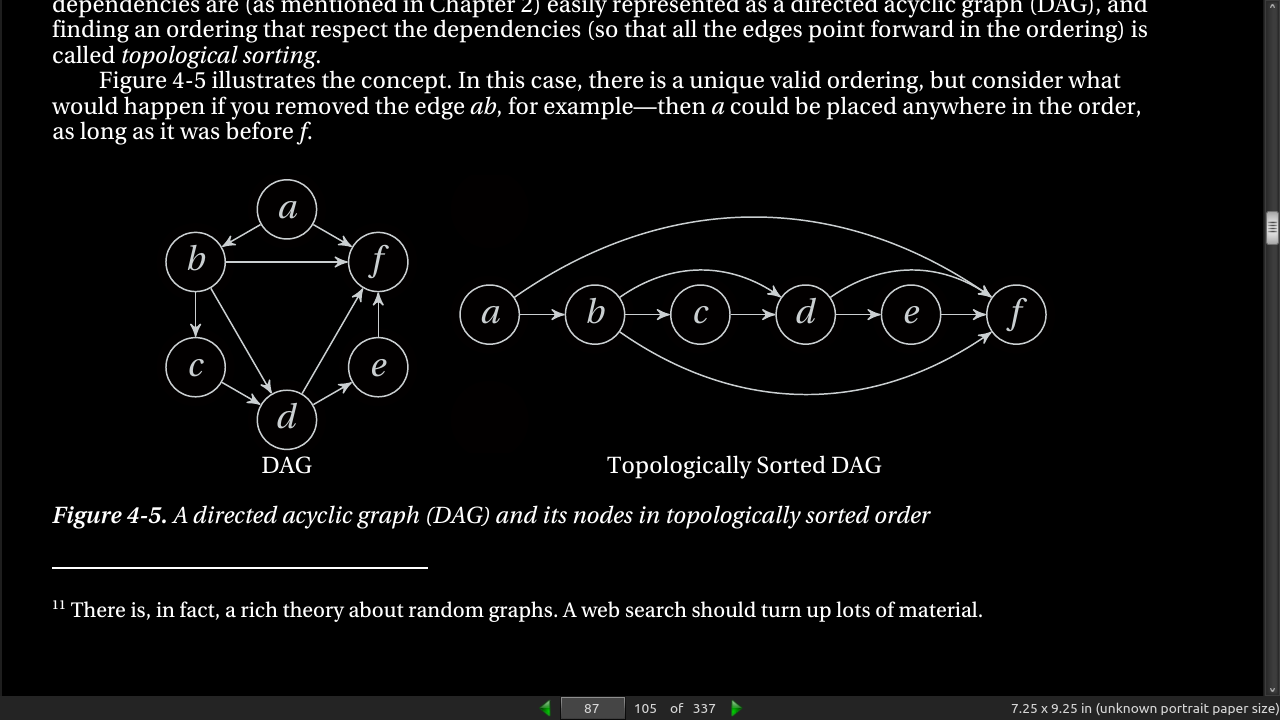
Such dependencies are (as mentioned in Chapter 2) easily represented as a directed acyclic graph (DAG), and finding an ordering that respect the dependencies (so that all the edges point forward in the ordering) is called topological sorting. Figure 4-5 illustrates the concept.
page 88:
- Tip If you’re using a Unix system of some sort, you can play around with topological sorting of graphs described in plain-text files, using the tsort command.
page 89:
- Tip If a problem reminds you of a problem or an algorithm you already know, that’s probably a good sign. In fact, building a mental archive of problems and algorithms is one of the things that can make you a skilled algorist. If you’re faced with a problem and you have no immediate associations, you could systematically consider any relevant (or semirelevant) techniques you know and look for reduction potential.
page 91:
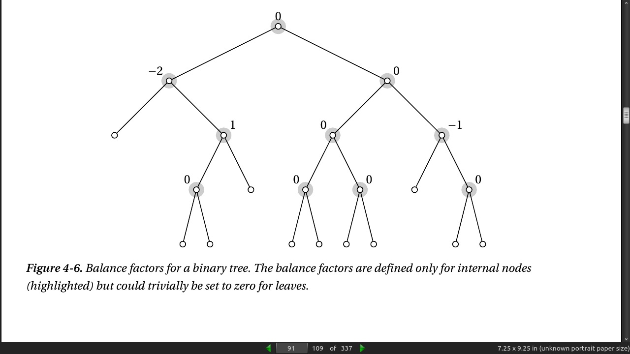
- A balance factor is defined for each internal node and is set to the difference between the heights of the left and right subtrees, where height is the greatest distance from the node (downward) to a leaf. For example, the left child of the root in Figure 4-6 has a balance factor of –2 because its left subtree is a leaf (with a height of 0), while its right child has a height of 2.
page 93:
- relaxation. You are in an airport, and you can reach several other airports by plane. From each of those airports, you can take the train to several towns and cities. Let’s say that you have a dict or list of flight times, A, so that A[u] is the time it will take you to get to airport u. Similarly, B[u][v] will give you the time it takes to get from airport u to town v by train. (B can be a list of lists or a dict of dicts, for example; see Chapter 2). Consider the following randomized way of estimating the time it will take you to get to each town, C[v]:
for v in range(n):
  C[v] = float('inf')
for i in range(N):
  u, v = randrange(n), randrange(n)
  C[v] = min(C[v], A[u] + B[u][v]) # Relax
- The idea here is to repeatedly see whether we can improve our estimate for C[v] by choosing another route. First go to u by plane, and then you take the train to v. If that gives us a better total time, we update C. As long as N is really large, we will eventually get the right answer for every town.
page 95:
-
If you can (easily) reduce A to B, then B is at least as hard as A.
-
If you want to show that X is hard and you know that Y is hard, reduce Y to X.
page 97:
- 4-1. A graph that you can draw in the plane without any edges crossing each other is called planar. Such a drawing will have a number of regions, areas bounded by the edges of the graph, as well as the (infinitely large) area around the graph. If the graph has V, E, and F nodes, edges, and regions, respectively, Euler’s formula for connected planar graphs says that V – E + F =
- Prove that this is correct using induction.
- 4-4. A node is called central if the greatest (unweighted) distance from that node to any other in the same graph is minimum. That is, if you sort the nodes by their greatest distance to any other node, the central nodes will be at the beginning.
· Chapter 5: Traversal: The Skeleton Key of Algorithmics
page 104:
- Listing 5-1. Walking Through a Connected Component of a Graph Represented Using Adjacency Sets
def walk(G, s, S=set()):            # Walk the graph from node s
  P, Q = dict(), set()              # Predecessors + "to do" queue
  P[s] = None                       # s has no predecessor
  Q.add(s)                          # We plan on starting with s
  while Q:                          # Still nodes to visit
    u = Q.pop()                     # Pick one, arbitrarily
    for v in G[u].difference(P, S): # New nodes?
      Q.add(v)                      # We plan to visit them!
      P[v] = u                      # Remember where we came from
  return P                          # The traversal tree
-
Tip Objects of the set type let you perform set operations on other types as well! For example, in Listing 5-1, I use the dict P as if it were a set (of its keys) in the difference method. This works with other iterables too, such as list or deque, for example, and with other set methods, such as update.
-
The S parameter Basically, it represents a “forbidden zone”—a set of nodes that we may not have visited during our traversal but that we have been told to avoid. As for the dictionary P, I’m using it to represent predecessors. Each time we add a new node to the queue, I set its predecessor; that is, I make sure I remember where I came from when I found it. These predecessors will, when taken together, form the traversal tree. If you don’t care about the tree, you’re certainly free to use a set of visited nodes instead .
-
Note Whether you add nodes to this sort of “visited” set at the same time as adding them to the queue or later, when you pop them from the queue, is generally not important. It does have consequences for where you need to add an “if visited …” check, though.
page 105:
- Listing 5-2. Finding Connected Components
def components(G):          # The connected components
  comp = []
  seen = set()              # Nodes we've already seen
  for u in G:               # Try every starting point
    if u in seen: continue  # Seen? Ignore it
    C = walk(G, u)          # Traverse component
    seen.update(C)          # Add keys of C to seen
    comp.append(C)          # Collect the components
  return comp
- The walk function returns a predecessor map (traversal tree) for the nodes it has visited, and I collect those in the comp list (of connected components). I use the seen set to make sure I don’t traverse from a node in one of the earlier components. Note that even though the operation seen.update(C) is linear in the size of C, the call to walk has already done the same amount of work, so asymptotically, it doesn’t cost us anything. All in all, finding the components like this is Θ(E + V), because every edge and node has to be explored.4 The walk function doesn’t really do all that much. Still, in many ways, this simple piece of code is the backbone of this chapter and (as the chapter title says) a skeleton key to understanding many of the other algorithms you’re going to learn. It might be worth studying it a bit.
page 108:
page 110:
-
Trémaux’s algorithm. In this formulation, it is commonly known as depth-first search, and it is one of the most fundamental (and fundamentally important) traversal algorithms.
-
Listing 5-4. Recursive Depth-First Search
def rec_dfs(G, s, S=None):
  if S is None: S = set()  # Initialize the history
  S.add(s)                 # We've visited s
  for u in G[s]:           # Explore neighbors
    if u in S: continue    # Already visited: Skip
    rec_dfs(G, u, S)       # New: Explore recursively
- [In depth first search] Once we start working with one node, we make sure we traverse all other nodes we can reach from it before moving on.
page 111:
def iter_dfs(G, s):
  S, Q = set(), []      # Visited-set and queue
  Q.append(s)           # We plan on visiting s
  while Q:              # Planned nodes left?
    u = Q.pop()         # Get one
    if u in S: continue # Already visited? Skip it
    S.add(u)            # We've visited it now
    Q.extend(G[u])      # Schedule all neighbors
    yield u             # Report u as visited
- use of a stack (a last-in, first-out or LIFO queue, here implemented by a list, using append and pop), the queue is not a set, so we risk having the same node scheduled for more than one visit. solved by checking a node for membership in S before adding its neighbors. added a yield statement, which will let you iterate over the graph nodes in DFS order. For example, if you had the graph from Figure 2-3 in the variable G, you could try the following:
>>> list(iter_dfs(G, 0))
[0, 5, 7, 6, 2, 3, 4, 1]
- both DFS and the other traversal algorithms work just as well for directed graphs. However, if you use DFS on a directed graph, you can’t expect it to explore an entire connected component. For example, for the graph in Figure 2-3, traversing from any other start node than “a” would mean that “a” would never be seen, because it has no in-edges.
page 112:
- Listing 5-6. A General Graph Traversal Function
def traverse(G, s, qtype=set):
  S, Q = set(), qtype()
  Q.add(s)
  while Q:
    u = Q.pop()
    if u in S: continue
    S.add(u)
    for v in G[u]:
      Q.add(v)
    yield u
>>> list(traverse(G, 0, stack))
[0, 5, 7, 6, 2, 3, 4, 1]
-
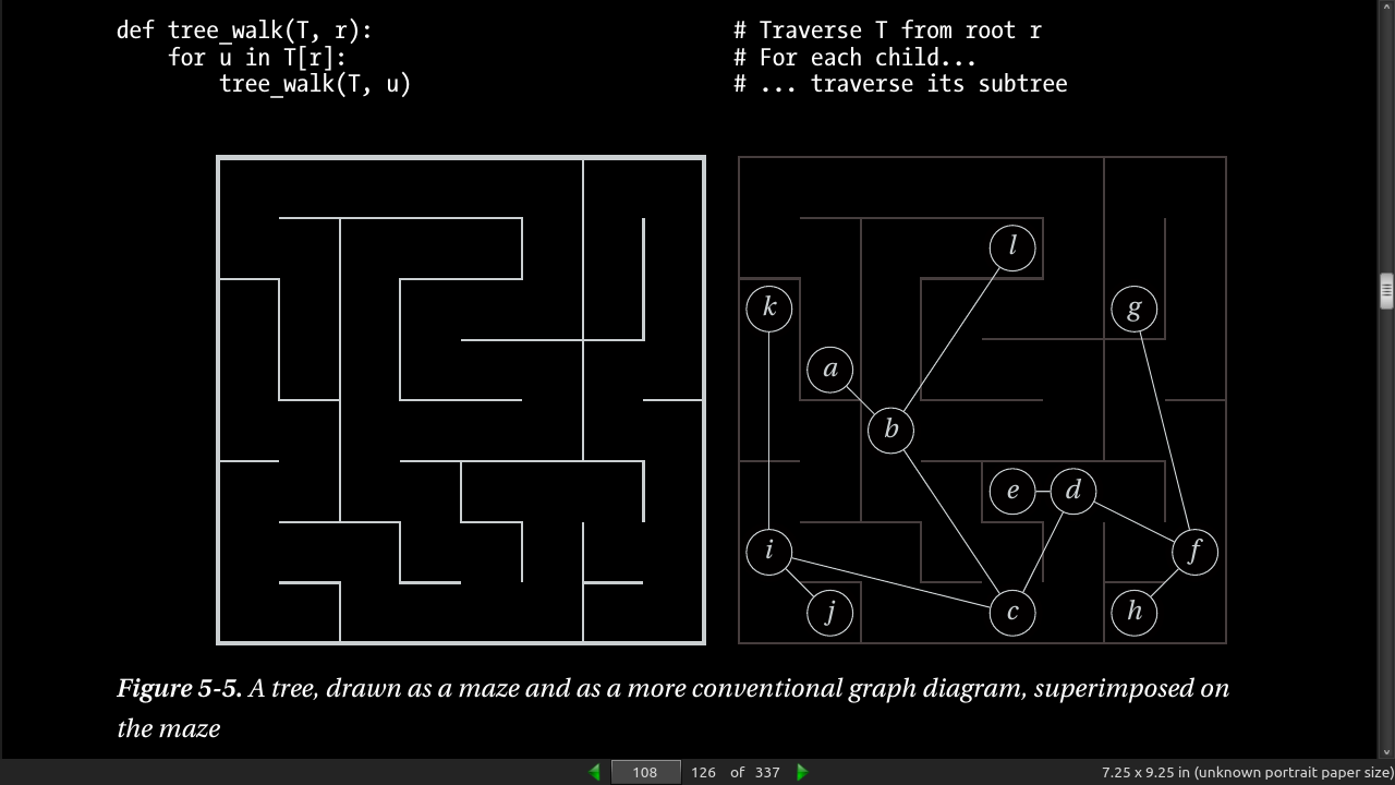
a traversal without cycles naturally forms a tree.
-
Listing 5-6. Depth-First Search with Timestamps
def dfs(G, s, d, f, S=None, t=0):
  if S is None: S = set()     # Initialize the history
  d[s] = t; t += 1            # Set discover time
  S.add(s)                    # We've visited s
  for u in G[s]:              # Explore neighbors
    if u in S: continue       # Already visited. Skip
    t = dfs(G, u, d, f, S, t) # Recurse; update timestamp
  f[s] = t; t += 1            # Set finish time
  return t                    # Return timestamp
page 113:
- If we perform DFS on a DAG, we could simply sort the nodes based on their descending finish times, and they’d be topologically sorted
page 114:
- If we’re looking for the shortest paths (disregarding edge weights, for now) from our start node to all the others, DFS will, most likely, give us the wrong answer.
page 115:

page 116:
- Listing 5-8. Iterative Deepening Depth-First Search
def iddfs(G, s):
  yielded = set()                     # Visited for the first time
  def recurse(G, s, d, S=None):       # Depth-limited DFS
    if s not in yielded:
      yield s
      yielded.add(s)
    if d == 0: return                 # Max depth zero: Backtrack
    if S is None: S = set()
    S.add(s)
    for u in G[s]:
      if u in S: continue
      for v in recurse(G, u, d-1, S): # Recurse with depth-1
        yield v
  n = len(G)
  for d in range(n):                  # Try all depths 0..V-1
    if len(yielded) == n: break       # All nodes seen?
  for u in recurse(G, s, d):
    yield u
- the only salient difference [in BFS] from DFS: we’ve replaced LIFO with FIFO.
page 117:
- Listing 5-9. Breadth-First Search
def bfs(G, s):
  P, Q = {s: None}, deque([s]) # Parents and FIFO queue
  while Q:
    u = Q.popleft()            # Constant-time for deque
    for v in G[u]:
      if v in P: continue      # Already has parent
      P[v] = u                 # Reached from u: u is parent
      Q.append(v)
  return P
-
5-9 is similar to 5-5. Deque over list.
-
To extract a path to a node u, you can simply “walk backward” in P:
>>> path = [u]
>>> while P[u] is not None:
...     path.append(P[u])
...     u = P[u]
...
>>> path.reverse()
- Tip One way of visualizing BFS and DFS is as browsing the Web. DFS is what you get if you keep following links and then use the Back button once you’re done with a page. The backtracking is a bit like an “undo.” BFS is more like opening every link in a new window (or tab) behind those you already have and then closing the windows as you finish with each page.
page 118:
-
Python has a deque class in the collections module in the standard library. In addition to methods such as append, extend, and pop, which are performed on the right side, it has left equivalents, called appendleft , extendleft, and popleft. Internally, the deque is implemented as a doubly linked list of blocks, each of which is an array of individual elements.
-
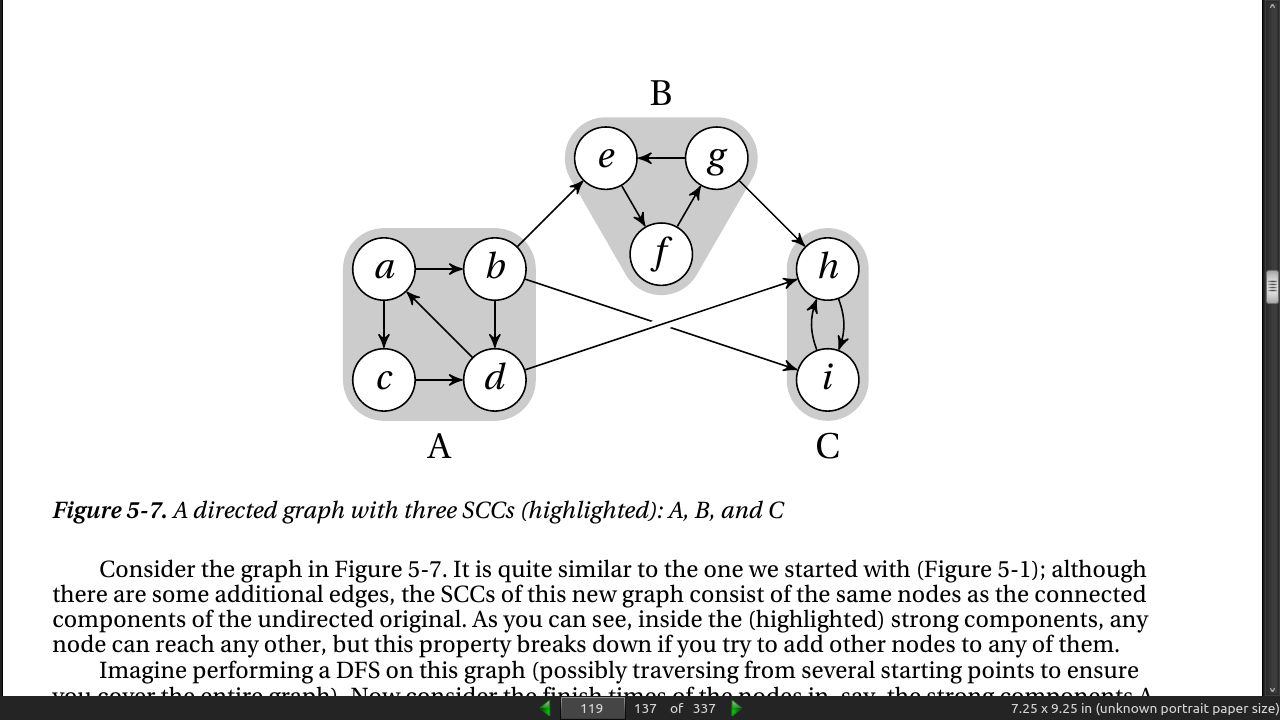
A connected component is a maximal subgraph where all nodes can reach each other if you ignore edge directions (or if the graph is undirected). To get strongly connected components, though, you need to follow the edge directions; so, SCCs are the maximal subgraphs where there is a directed path from any node to any other.
page 119:
page 120:
- Listing 5-10. Kosaraju’s Algorithm for Finding Strongly Connected Components
def tr(G):                  # Transpose (rev. edges of) G
  GT = {}
  for u in G: GT[u] = set() # Get all the nodes in there
  for u in G:
    for v in G[u]:
      GT[v].add(u)          # Add all reverse edges
  return GT

def scc(G):
  GT = tr(G)                # Get the transposed graph
  sccs, seen = [], set()
  for u in dfs_topsort(G):  # DFS starting points
    if u in seen: continue  # Ignore covered nodes
      C = walk(GT, u, seen) # Don't go "backward" (seen)
      seen.update(C)        # We've now seen C
      sccs.append(C)        # Another SCC found
  return sccs
- If you try running scc on the graph in Figure 5-7, you should get the three sets {a, b, c, d}; {e, f, g}; and {i, h}.
· Chapter 6: Divide, Combine, and Conquer
page 126:
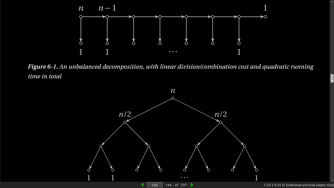
- Using weak induction generates a recurrance like T(n) = T(n-1) + T(1) + n. Each reduces the problem size by 1 and ends up with quadratic running time. T(n) = 2T(n/2) + n is the equation for dividing the subproblems more evenly (not 1 each step, half). This runs in (n log n) time. See fig 6.1, 6.2.

page 127:
- Weak induction is 1 step at a time reduction and strong induction is divide and conquer?
page 128:
- Listing 6-1. A General Implementation of the Divide and Conquer Scheme
def divide_and_conquer(S, divide, combine):
  if len(S) == 1: return S
  L, R = divide(S)
  A = divide_and_conquer(L, divide, combine)
  B = divide_and_conquer(R, divide, combine)
  return combine(A, B)
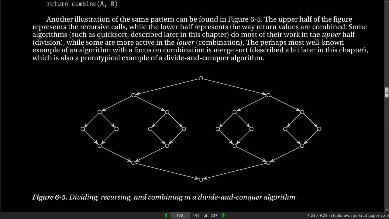
page 129:
- bisect module in standard library (written in C).
>>> from bisect import bisect
>>> a = [0, 2, 3, 5, 6, 8, 8, 9]
>>> bisect(a, 5)
4
- it doesn’t return the position of the 5 that’s already there. Rather, it reports the position to insert the new 5, making sure it’s placed after all existing items with the same value. In fact, bisect is another name for bisect_right, and there’s also a bisect_left
page 131:

page 133:
- Listing 6-2. Insertion into and Search in a Binary Search Tree
class Node:
  lft = None
  rgt = None
  def __init__(self, key, val):
    self.key = key
    self.val = val

  def insert(node, key, val):
    if node is None: return Node(key, val)  # Empty leaf: it's not here
    if node.key == key: node.val = val      # Found key: return val
    elif key < node.key:                    # Less than the key?
      node.lft = insert(node.lft, key, val) # Go left
    else:                                   # Otherwise...
      node.rgt = insert(node.rgt, key, val) # Go right
  return node

  def search(node, key):
    if node is None: raise KeyError         # Empty leaf: add node here
    if node.key == key: return node.val     # Found key: replace val
    elif key < node.key:                    # Less than the key?
      return search(node.lft, key)          # Go left
    else:                                   # Otherwise...
      return search(node.rgt, key)          # Go right

class Tree:                                 # Simple wrapper
  root = None
  def __setitem__(self, key, val):
    self.root = insert(self.root, key, val)

  def __getitem__(self, key):
    return search(self.root, key)

  def __contains__(self, key):
    try: search(self.root, key)
    except KeyError: return False
    return True
- Using it:
>>> tree = Tree()
>>> tree["a"] = 42
>>> tree["a"]
42
>>> "b" in tree
False
-
Note The implementation in Listing 6-2 does not permit the tree to contain duplicate keys. If you insert a new value with an existing key, the old value is simply overwritten. This could easily be changed, because the tree structure itself does not preclude duplicates.
-
Bisection is fast, with little overhead, but works only on sorted arrays (such as Python lists). And sorted arrays are hard to maintain; adding elements takes linear time.
-
Search trees have more overhead but are dynamic and let you insert and remove elements.
-
In many cases, though, the clear winner will be the hash table, in the form of dict. Its average asymptotic running time is constant (as opposed to the logarithmic running time of bisection and search trees), and it is very close to that in practice, with little overhead.
-
search trees will let you access your values in sorted order—either all of them or just a portion.
-
Trees can also be extended to work in multiple dimensions, where hashing may be hard to achieve.
-
if you want the entry that is closest to your lookup key, a search tree would be the way to go.
-
Actually, more flexible may not be entirely correct. There are many objects (such as complex numbers) that can be hashed but that cannot be compared for size.
page 134:
-
Tip If you’re looking for the k smallest (or largest) objects in an iterable in Python, you would probably use the nsmallest (or nlargest) function from the heapq module if your k is small, relative to the total number of objects. If the k is large, you should probably sort the sequence (either using the sort method or using the sorted function) and pick out the k first objects.
-
Listing 6-3. A Straightforward Implementation of Partition and Select
def partition(seq):
  pi, seq = seq[0], seq[1:]        # Pick and remove the pivot
  lo = [x for x in seq if x <= pi] # All the small elements
  hi = [x for x in seq if x > pi]  # All the large ones
  return lo, pi, hi                # pi is "in the right place"

def select(seq, k):
  lo, pi, hi = partition(seq)      # [<= pi], pi, [> pi]
  m = len(lo)
  if m == k: return pi             # We found the kth smalles
  elif m < k:                      # Too far to the left
    return select(hi, k-m-1)       # Remember to adjust k
  else:                            # Too far to the right
    return select(lo, k)           # Just use original k here
page 137:
- Timsort is a close relative to merge sort. It’s an in-place algorithm, in that it merges segments and leaves the result in the original array (although it uses some auxiliary memory during the merging). Instead of simply sorting the array half-and-half and then merging those, though, it starts at the beginning, looking for segments that are already sorted (possibly in reverse), called runs. In random arrays, there won’t be many, but in many kinds of real data, there may be a lot—giving the algorithm a clear edge over a plain merge sort and a linear running time in the best case (and that covers a lot of cases beyond simply getting a sequence that’s already sorted).
page 138:
- lg(n!) is asymptotically equivalent to n*lg(n) I think lg here is natural log
page 140:
- A region is convex if you can draw a line between any two points inside it, and the line stays inside the region.
page 144:
- Note The 2-3-tree is a special case of the B-tree, which forms the basis of almost all database systems, and disk-based trees used in such diverse areas as geographic information systems and image retrieval. The important extension is that B-trees can have thousands of keys (and subtrees), and each node is usually stored as a contiguous block on disk. The main motivation for the large blocks is to minimize the number of disk accesses.

page 147:
- BLACK BOX: BINARY HEAPS, HEAPQ, AND HEAPSORT
page 149:
- If you like bisection, you should look up interpolation search, which for uniformly distributed data has an average-case running time of O(lg lg n). For implementing sets (that is, efficient membership checking) other than sorted sequences, search trees and hash tables, you could have a look at Bloom filters. If you like search trees and related structures, there are lots of them out there. You could find tons of different balancing mechanisms (red black trees, AVL-trees, splay trees), some of them randomized (treaps), and some of them only abstractly representing trees (skip lists). There are also whole families of specialized tree structures for indexing multidimensional coordinates (so-called spatial access methods) and distances (metric access methods). Other trees structures to check out are interval trees, quadtrees, and octtrees.
· Chapter 7: Greed Is Good? Prove It!
page 151:
- So-called greedy algorithms are short-sighted, in that they make each choice in isolation, doing what looks good right here, right now. In many ways, eager or impatient might be better names for them,
page 153:
- Making change, denom is $10-0.01, owed in cents. It works but is brittle. Reordering denom or different currencies break it.
>>> denom = [10000, 5000, 2000, 1000, 500, 200, 100, 50, 25, 10, 5, 1]
>>> owed = 56329
>>> payed = []
>>> for d in denom:
...   while owed >= d:
...   owed -= d
...   payed.append(d)
...
>>> sum(payed)
56329
>>> len(payed)
14
page 156:
- If we view each object individually, this is often called 0-1 knapsack, because we can take 0 or 1 of each object.
page 157:
-
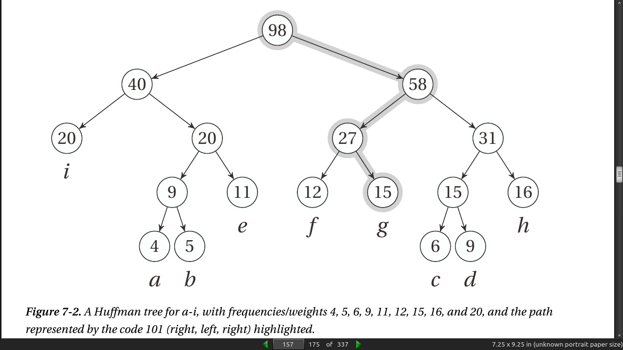
Your goal for the tree structure is still the same. How can you minimize the sum of depth(u) × weight(u) over all leaves u? This problem certainly has other applications as well. In fact, the original (and most common) application is compression—representing a text more compactly—through variable-length codes.
-
let a partial solution consist of several tree fragments and then repeatedly combine them. When we combine two trees, we add a new, shared root and give it a weight equal to the sum of its children (that is, the previous roots). This is exactly what the numbers inside the nodes in Figure 7-2 mean.
page 158:
- Listing 7-1. Huffman’s Algorithm
from heapq import heapify, heappush, heappop
from itertools import count
def huffman(seq, frq):
  num = count()
  trees = list(zip(frq, num, seq))      # num ensures valid ordering
  heapify(trees)                        # A min-heap based on freq
  while len(trees) > 1:                 # Until all are combined
    fa, _, a = heappop(trees)           # Get the two smallest trees
    fb, _, b = heappop(trees)
    n = next(num)
    heappush(trees, (fa+fb, n, [a, b])) # Combine and re-add them
  return trees[0][-1]
- If a future version of the heapq library lets you use a key function, such as in list.sort, you’d no longer need this tuple wrapping at all, of course.
page 159:
- Here’s an example of how you might use the code:
>>> seq = "abcdefghi"
>>> frq = [4, 5, 6, 9, 11, 12, 15, 16, 20]
>>> huffman(seq, frq)
[['i', [['a', 'b'], 'e']], [['f', 'g'], [['c', 'd'], 'h']]]
-
As you can see, the resulting tree structure is equivalent to the one shown in Figure 7-2.
-
Listing 7-2. Extracting Huffman Codes from a Huffman Tree
def codes(tree, prefix=""):
  if len(tree) == 1:
    yield (tree, prefix) # A leaf with its code
    return
  for bit, child in zip("01", tree): # Left (0) and right (1)
for pair in codes(child, prefix + bit): # Get codes recursively
  yield pair
- The codes function yields (char, code) pairs suitable for use in the dict constructor, for example. To use such a dict to compress a code, you’d just iterate over the text and look up each character. To decompress the text, you’d rather use the Huffman tree directly, traversing it using the bits in the input for directions (that is, determining whether you should go left or right); I’ll leave the details as an exercise for the reader.
page 161:
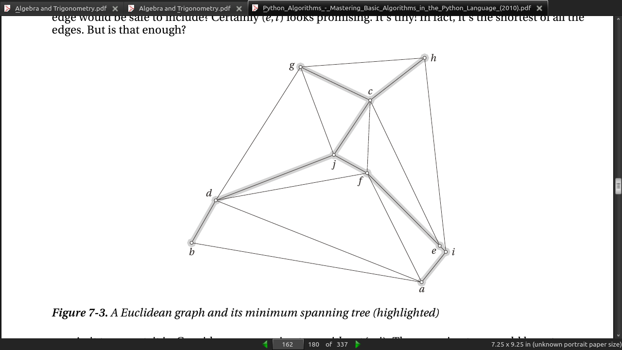
- [A Minimum Spanning Tree] could be useful in building an electrical grid, building the core of a road or railroad network, laying out a circuit, or even performing some forms of clustering (where we’d only almost connect all the nodes).
page 162:
page 165:
- Listing 7-4. Kruskal’s Algorithm (minimum spanning tree)
def find(C, u):
  if C[u] != u:
    C[u] = find(C, C[u]) # Path compression
  return C[u]

def union(C, R, u, v):a
  u, v = find(C, u), find(C, v)
  if R[u] > R[v]: # Union by rank
    C[v] = u
  else:
    C[u] = v
  if R[u] == R[v]: # A tie: Move v up a level
    R[v] += 1

def kruskal(G):
  E = [(G[u][v],u,v) for u in G for v in G[u]]
  T = set()
  C, R = {u:u for u in G}, {u:0 for u in G} # Comp. reps and ranks
  for _, u, v in sorted(E):
    if find(C, u) != find(C, v):
      T.add((u, v))
      union(C, R, u, v)
  return T
- find() above is making sure each node is not already in the subsolution.
page 167:
- Listing 7-5. Prim’s Algorithm
from heapq import heappop, heappush
def prim(G, s):
  P, Q = {}, [(0, None, s)]
  while Q:
    _, p, u = heappop(Q)
    if u in P:  #if we already added u to P, don't add a dupe
      continue
    P[u] = p
    for v, w in G[u].items():
      heappush(Q, (w, u, v))
  return P
- prim() above adds duplicate nodes with different weights and discards duplicate heavier edges (u in P: continue).
page 168:
-
Graham and Hell succinctly explain the algorithms as follows. A partial solution is a spanning forest, consisting of a set of fragments (components, trees). Initially, each node is a fragment. In each iteration, edges are added, joining fragments, until we have a spanning tree.
-
Algorithm 1: Add a shortest edge that joins two different fragments.
-
Algorithm 2: Add a shortest edge that joins the fragment containing the root to another fragment.
-
Algorithm 3: For every fragment, add the shortest edge that joins it to another fragment.
-
For algorithm 2, the root is chosen arbitrarily at the beginning. For algorithm 3, it is assumed that all edge weights are different to ensure that no cycles can occur. As you can see, all three algorithms are based on the same fundamental fact—that the shortest edge over a cut is safe. Also, in order to implement them efficiently, you need to be able to find shortest edges, detect whether two nodes belong to the same fragment, and so forth (as explained for algorithms 1 and 2 in the main text). Still, these brief explanations can be useful as a memory aid or to get the bird’s-eye perspective on what’s going on.
page 172:
-
Greedy algorithms take the best element at any given step, without reguard for previous/later choices.
-
Often easy to write, hard to prove they are optimal. Often prove by “keeping up”.
-
Important greedy problems and algorithms discussed in this chapter include the knapsack problem (selecting a weight-bounded subset of items with maximum value), where the fractional version can be solved greedily; Huffman trees, which can be used to create optimal prefix codes, and are built greedily by combining the smallest trees in the partial solution; and minimum spanning trees, which can be built using Kruskal’s algorithm (keep adding the smallest valid edge) or Prim’s algorithm (keep connecting the node that is closest to your tree).
· Chapter 8: Tangled Dependencies and Memoization
page 175:
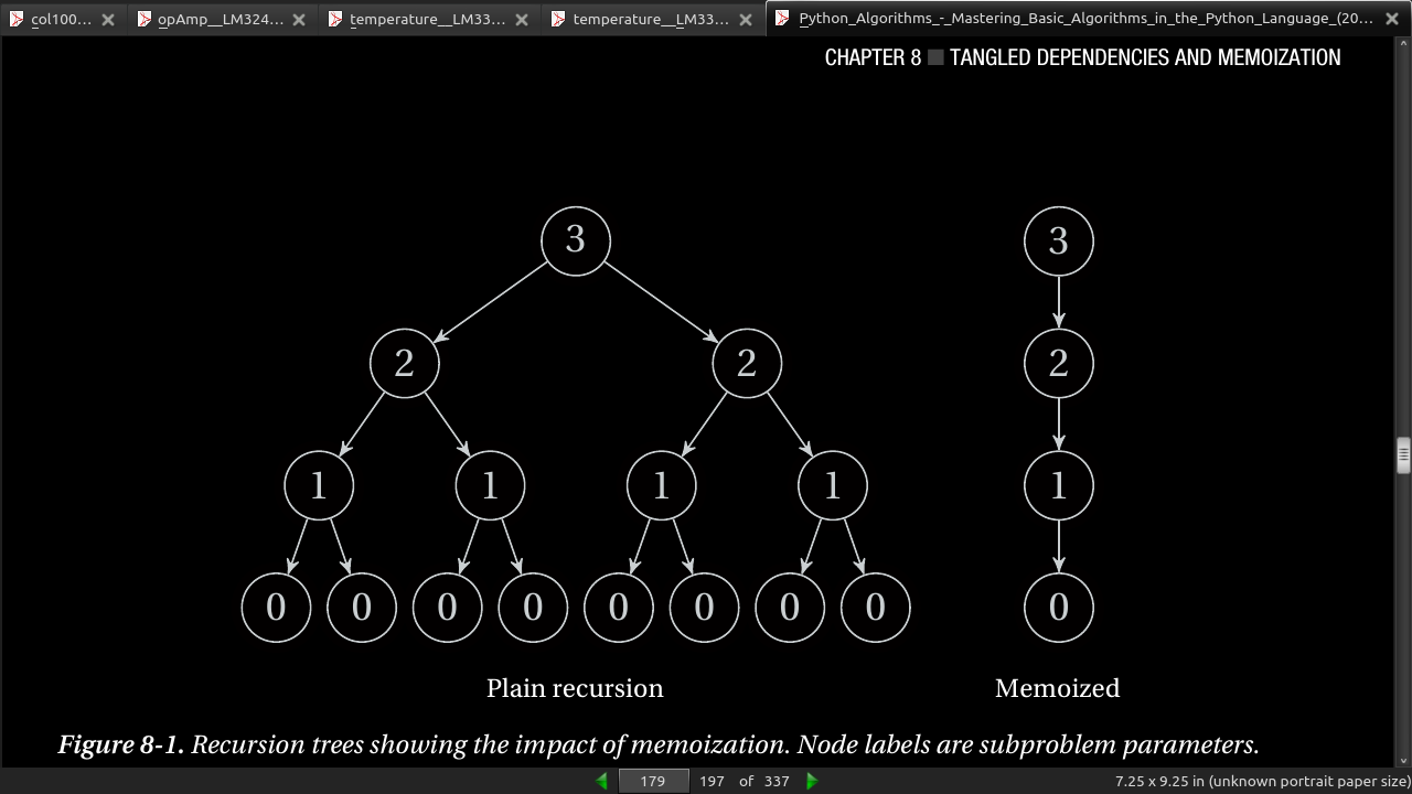
- Another option—one I think is particularly suited to high-level languages such as Python—is to implement the recursive formulation directly but to cache the return values. If a call is made more than once with the same arguments, the result is simply returned directly from the cache. This is called memoization.
page 176:
- Listing 8-1. A Naïve Solution to the Longest Increasing Subsequence Problem
from itertools import combinations
def naive_lis(seq):
  for length in range(len(seq), 0, -1):    # n, n-1, ... , 1
    for sub in combinations(seq, length):  # Subsequences of given length
      if list(sub) == sorted(sub):         # An increasing subsequence?
        return sub                         # Return it!
-
combinations from itertools. Generates combinations (!) from lists.
-
Algorithms should be DRY as well as code.
page 177:
- Listing 8-2. A Memoizing Decorator
from functools import wraps
def memo(func):
  cache = {}                       # Stored subproblem solutions
  @wraps(func)                     # Make wrap look like func
  def wrap(*args):                 # The memoized wrapper
    if args not in cache:          # Not already computed?
      cache[args] = func(*args)    # Compute & cache the solution
    return cache[args]             # Return the cached solution
  return wrap                      # Return the wrapper
- The idea of a memoized function4 is that it caches its return values. If you call it a second time with the same parameters, it will simply return the cached value. You can certainly put this sort of caching logic inside your function, but the memo function is a more reusable solution. It’s even designed to be used as a decorator.
page 178:
>>> @memo
... def fib(i):
... if i < 2: return 1
... return fib(i-1) + fib(i-2)
...
>>> fib(100)
573147844013817084101
- The main difference is that the subproblems have tangled dependencies. Or, to put it in another way: We’re faced with overlapping subproblems. This is perhaps even clearer in this rather silly relative of the Fibonacci numbers: a recursive formulation of the powers of two:
>>> def two_pow(i):
... if i == 0: return 1
... return two_pow(i-1) + two_pow(i-1)
...
>>> two_pow(10)
1024
>>> two_pow(100) #hangs
- Still horrible. Try adding @memo, and you’ll get the answer instantly. Or, you could try to make the following change, which is actually equivalent:
>>> def two_pow(i):
... if i == 0: return 1
... return 2*two_pow(i-1)
...
>>> print(two_pow(10))
1024
>>> print(two_pow(100))
1267650600228229401496703205376
page 179:
(n) = (n-1) + (n-1) n choose k (k) (k-1) (k)
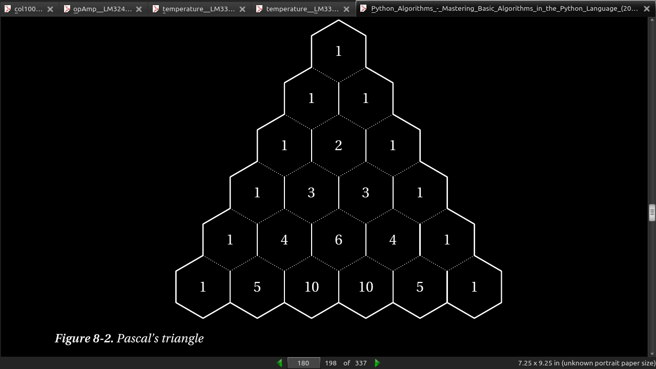
- Figure 8-2 shows how the binomial coefficients can be placed in a triangular pattern so that each number is the sum of the two above it. This means that the row (counting from zero) corresponds to n, and the column (the number of the cell, counting from zero at the left in its row) corresponds to k. For example, the value 6 corresponds to C(4, 2), and can be calculated as C(3,1) + C(3,2) = 3 + 3 = 6.
page 180:
- The code for C(n, k) is trivial:
>>> @memo
>>> def C(n,k):
... if k == 0: return 1
... if n == 0: return 0
... return C(n-1,k-1) + C(n-1,k)
>>> C(4,2)
6
>>> C(10,7)
120
>>> C(100,50)
100891344545564193334812497256
page 181:
- Let’s reverse our algorithm, filling out Pascal’s triangle directly. To keep things simple, I’ll use a defaultdict as the cache; feel free to use nested lists, for example. (See also Exercise 8-4.)
>>> from collections import defaultdict
>>> n, k = 10, 7
>>> C = defaultdict(int)
>>> for row in range(n+1):
... C[row,0] = 1
... for col in range(1,k+1):
... C[row,col] = C[row-1,col-1] + C[row-1,col]
...
>>> C[n,k]
120
-
Basically the same thing is going on. The main difference is that we need to figure out which cells in the cache need to be filled out, and we need to find a safe order to do it in so that when we’re about to calculate C[row,col], the cells C[row-1,col-1] and C[row-1,col] are already calculated. With the memoized function, we needn’t worry about either issue: it will calculate whatever it needs recursively.
-
One useful way to visualize dynamic programming algorithms with one or two subproblem parameters (such as n and k, here) is to use a (real or imagined) spreadsheet. For example, try calculating binomial coefficients in a spreadsheet by filling the first column with ones and filling in the rest of the first row with zeros. Put the formula =A1+B1 into cell B2, and copy it to the remaining cells.
page 183:
- Listing 8-3. Recursive, Memoized DAG Shortest Path
def rec_dag_sp(W, s, t):                   # Shortest path from s to t
  @memo # Memoize f
  def d(u): # Distance from u to t
    if u == t:
      return 0                             # We're there!
    return min(W[u][v]+d(v) for v in W[u]) # Best of every first step
return d(s)
- Listing 8-4. DAG Shortest Path
def dag_sp(W, s, t):
  d = {u:float('inf') for u in W}
  d[s] = 0
  for u in topsort(W):
    if u == t: break
    for v in W[u]:
      d[v] = min(d[v], d[u] + W[u][v])
  return d[t]
page 185:
- Listing 8-5. A Memoized Recursive Solution to the Longest Increasing Subsequence Problem
def rec_lis(seq):                           # Longest increasing subseq.
  @memo
  def L(cur):                               # Longest ending at seq[cur]
    res = 1                                 # Length is at least 1
    for pre in range(cur):                  # Potential predecessors
      if seq[pre] <= seq[cur]:              # A valid (smaller) predec.
        res = max(res, 1 + L(pre))          # Can we improve the solution?
    return res
  return max(L(i) for i in range(len(seq))) # The longest of them all
- Listing 8-6. A Basic Iterative Solution to the Longest Increasing Subsequence Problem
def basic_lis(seq):
  L = [1] * len(seq)
  for cur, val in enumerate(seq):
    for pre in range(cur):
      if seq[pre] <= val:
        L[cur] = max(L[cur], 1 + L[pre])
  return max(L)
page 187:
- Listing 8-7. Longest Increasing Subsequence
from bisect import bisect
def lis(seq):                         # Longest increasing subseq.
  end = []                            # End-values for all lengths
  for val in seq:                     # Try every value, in order
  idx = bisect(end, val)              # Can we build on an end val?
  if idx == len(end): end.append(val) # Longest seq. extended
  else: end[idx] = val                # Prev. endpoint reduced
  return len(end)                     # The longest we found
- if the length of the sequences are m and n and the length of the longest common subsequence is k, the edit distance is m + n - 2k.
page 188:
- Listing 8-8. A Memoized Recursive Solution to the LCS Problem
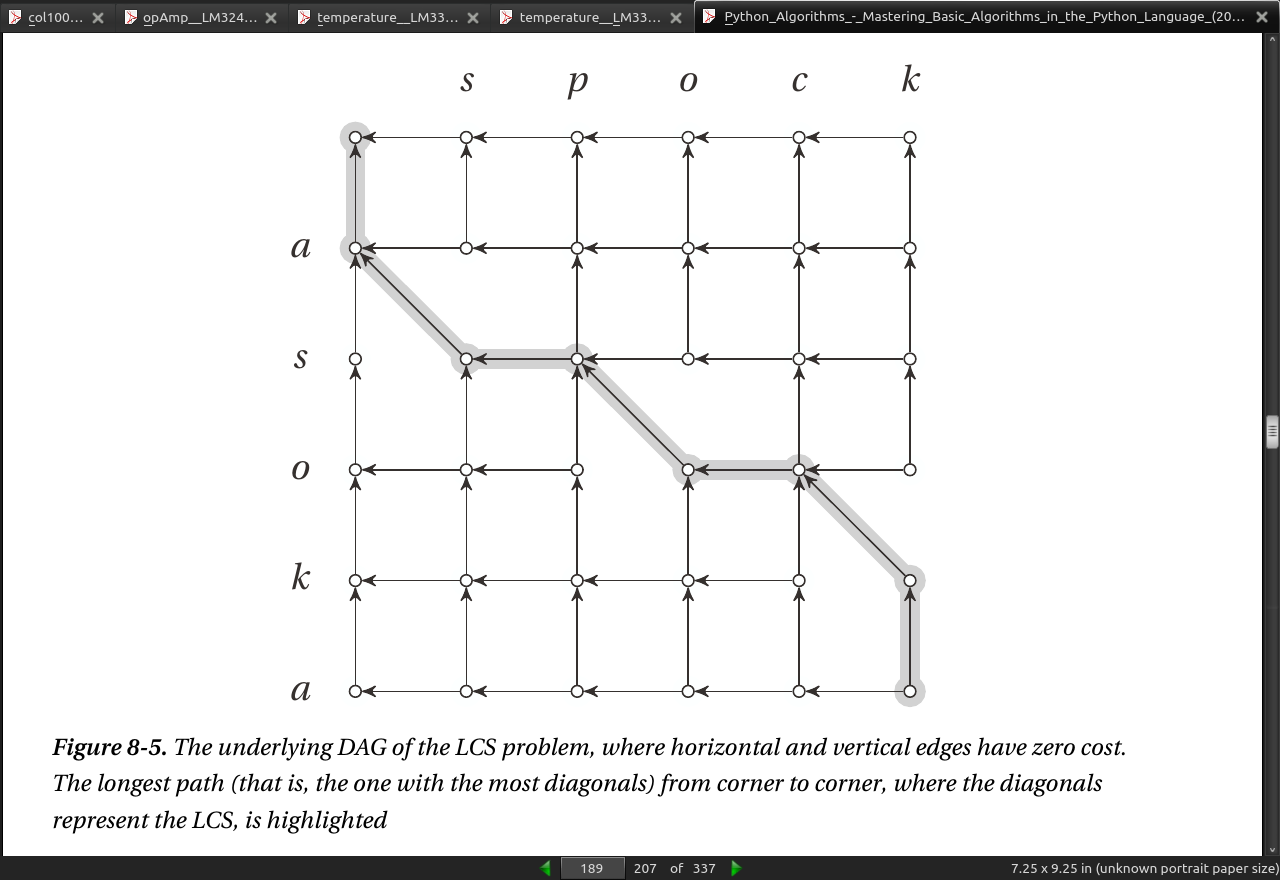
def rec_lcs(a,b):                          # Longest common subsequence
  @memo # L is memoized
  def L(i,j):                              # Prefixes a[:i] and b[:j]
    if min(i,j) < 0: return 0              # One prefix is empty
    if a[i] == b[j]: return 1 + L(i-1,j-1) # Match! Move diagonally
    return max(L(i-1,j), L(i,j-1))         # Chop off either a[i] or b[j]
  return L(len(a)-1,len(b)-1)              # Run L on entire sequences
page 189:
- Listing 8-9. An Iterative Solution to the Longest Common Subsequence (LCS)
def lcs(a,b):
  n, m = len(a), len(b)
  pre, cur = [0]*(n+1), [0]*(n+1)      # Previous/current row
  for j in range(1,m+1):               # Iterate over b
    pre, cur = cur, pre                # Keep prev., overwrite cur.
    for i in range(1,n+1):             # Iterate over a
      if a[i-1] == b[j-1]:             # Last elts. of pref. equal?
        cur[i] = pre[i-1] + 1          # L(i,j) = L(i-1,j-1) + 1
      else:                            # Otherwise...
        cur[i] = max(pre[i], cur[i-1]) # max(L(i,j-1),L(i-1,j))
  return cur[n] # L(n,m)
page 190:
- Listing 8-10. A Memoized Recursive Solution to the Unbounded Integer Knapsack Problem
def rec_unbounded_knapsack(w, v, c): # Weights, values and capacity
  @memo                              # m is memoized
  def m(r):                          # Max val. w/remaining cap. r
    if r == 0: return 0              # No capacity? No value
    val = m(r-1)                     # Ignore the last cap. unit?
    for i, wi in enumerate(w):       # Try every object
      if wi > r: continue            # Too heavy? Ignore it
      val = max(val, v[i] + m(r-wi)) # Add value, remove weight
    return val                       # Max over all last objects
  return m(c)                        # Full capacity available
- The running time here depends on the capacity and the number of objects. Each memoized call m(r) is computed only once, which means that for a capacity c, we have Θ(c) calls. Each call goes through all the n objects, so the resulting running time is Θ(cn).
page 191:
- Listing 8-11. An Iterative Solution to the Unbounded Integer Knapsack Problem
def unbounded_knapsack(w, v, c):
  m = [0]
  for r in range(1,c+1):
    val = m[r-1]
    for i, wi in enumerate(w):
      if wi > r: continue
      val = max(val, v[i] + m[r-wi])
    m.append(val)
  return m[c]
page 192:
- Listing 8-12. A Memoized Recursive Solution to the 0-1 Knapsack Problem
def rec_knapsack(w, v, c):              # Weights, values and capacity
@memo                                   # m is memoized
def m(k, r):                            # Max val., k objs and cap r
if k == 0 or r == 0: return 0           # No objects/no capacity
i = k-1                                 # Object under consideration
drop = m(k-1, r)                        # What if we drop the object?
if w[i] > r: return drop                # Too heavy: Must drop it
return max(drop, v[i] + m(k-1, r-w[i])) # Include it? Max of in/out
return m(len(w), c)                     # All objects, all capacity
- Listing 8-13. An Iterative Solution to the 0-1 Knapsack Problem
def knapsack(w, v, c):                    # Returns solution matrices
  n = len(w)                              # Number of available items
  m = [[0]*(c+1) for i in range(n+1)]     # Empty max-value matrix
  P = [[False]*(c+1) for i in range(n+1)] # Empty keep/drop matrix
  for k in range(1,n+1):                  # We can use k first objects
    i = k-1                               # Object under consideration
    for r in range(1,c+1):                # Every positive capacity
      m[k][r] = drop = m[k-1][r]          # By default: drop the object
      if w[i] > r: continue               # Too heavy? Ignore it
      keep = v[i] + m[k-1][r-w[i]]        # Value of keeping it
      m[k][r] = max(drop, keep)           # Best of dropping and keeping
      P[k][r] = keep > drop               # Did we keep it?
  return m, P                             # Return full results
- Now that the knapsack function returns more information, we can use it to extract the set of objects actually included in the optimal solution. For example, you could do something like this:
>>> m, P = knapsack(w, v, c)
>>> k, r, items = len(w), c, set()
>>> while k > 0 and r > 0:
...   i = k-1
...   if P[k][r]:
...     items.add(i)
...     r -= w[i]
...   k -= 1
- In other words, by simply keeping some information about the choices made (in this case, keeping or dropping the element under consideration), we can gradually trace ourselves back from the final state to the initial conditions. In this case, I start with the last object and check P[k][r] to see whether it was included. If it was, I subtract its weight from r; if it wasn’t, I leave r alone (as we still have the full capacity available). In either case, I decrement k, because we’re done looking at the last element and now want to have a look at the next-to-last element (with the updated capacity). You might want to convince yourself that this backtracking operation has a linear running time. The same basic idea can be used in all the examples in this chapter.
page 196:
-
Problems solved using DP in this chapter include calculating binomial coefficients, finding shortest paths in DAGs, finding the longest increasing subsequence of a given sequence, finding the longest common subsequence of two given sequences, getting the most out of your knapsack with limited and unlimited supplies of indivisible items, and building binary search trees that minimize the expected lookup time.
-
For some sequence comparison goodness in the Python standard library, check out the difflib module. If you have Sage installed, you could have a look at its knapsack module (sage.numerical.knapsack).
· Chapter 9: From A to B with Edsger and Friends
page 200:
- Listing 9-1. The Relaxation Operation
inf = float('inf')
def relax(W, u, v, D, P):
  d = D.get(u,inf) + W[u][v] # Possible shortcut estimate
  if d < D.get(v,inf):       # Is it really a shortcut?
    D[v], P[v] = d, u        # Update estimate and parent
    return True              # There was a change!
- The idea is that we look for an improvement to the currently known distance to v by trying to take a shortcut through v. If it turns out not to be a shortcut, fine. We just ignore it. If it is a shortcut, we register the new distance and remember where we came from (by setting P[v] to u). I’ve also added a small extra piece of functionality: the return value indicates whether any change actually took place; that’ll come in handy later (though you won’t need it for all your algorithms). Here’s a look at how it works:
>>> D[u]
7
>>> D[v]
13
>>> W[u][v]
3
>>> relax(W, u, v, D, P)
True
>>> D[v]
10
>>> D[v] = 8
>>> relax(W, u, v, D, P)
>>> D[v]
8
- As you can see, the first call to relax improves D[v] from 13 to 10, because I found a shortcut through u, which I had (presumably) already reached using a distance of 7, and which was just 3 away from v. Now I somehow discover that I can reach v by a path of length 8. I run relax again, but this time, no shortcut is found, so nothing happens. As you can probably surmise, if I now set D[u] to 4 and ran the same relax again, D[v] would improve, this time to 7, propagating the improved estimate from u to v.
page 201:
- if you keep randomly relaxing forever, you know that you’ll have the right answer.
page 202:
- Tip Imagine each node continuously shouting out bids for supplying short paths to its out-neighbors, based on the shortest path it has gotten itself, so far. If any node gets a better offer than what it already has, it switches its path supplier and lowers its bids accordingly.
page 203:
- Listing 9-2. The Bellman-Ford Algorithm
def bellman_ford(G, s):
  D, P = {s:0}, {}                    # Zero-dist to s; no parents
  for rnd in G:                       # n = len(G) rounds
    changed = False                   # No changes in round so far
    for u in G:                       # For every from-node...
      for v in G[u]:                  # ... and its to-nodes...
        if relax(G, u, v, D, P):      # Shortcut to v from u?
          changed = True              # Yes! So something changed
    if not changed: break             # No change in round: Done
  else:                               # Not done before round n?
    raise ValueError('negative cycle')# Negative cycle detected
  return D, P                         # Otherwise: D and P correct
page 205:
- Listing 9-3. Dijkstra’s Algorithm
from heapq import heappush, heappop
def dijkstra(G, s):
  D, P, Q, S = {s:0}, {}, [(0,s)], set() # Est., tree, queue, visited
  while Q:                               # Still unprocessed nodes?
    _, u = heappop(Q)                    # Node with lowest estimate
    if u in S: continue                  # Already visited? Skip it
    S.add(u)                             # We've visited it now
    for v in G[u]:                       # Go through all its neighbors
      relax(G, u, v, D, P)               # Relax the out-edge
      heappush(Q, (D[v], v))             # Add to queue, w/est. as pri
  return D, P                            # Final D and P returned
- Dijkstra’s algorithm may be similar to Prim’s (with another set of priorities for the queue), but it is also closely related to another old favorite: BFS. Consider the case where the edge weights are positive integers. Now, replace an edge that has weight w with w -1 unweighted edges, connecting a path of dummy nodes (see Figure 9-2). We’re breaking what chances we had for an efficient solution (see Exercise 9-3), but we know that BFS will find a correct solution. In fact, it will do so in a way very similar to Dijkstra’s algorithm: it will spend an amount of time on each (original) edge proportional to its weight

page 206:
-
It’s a bit like you had set up a series of dominoes along each edge (the number of dominoes proportional to the weight), and you then tip the first domino in the start node. A node may be reached from multiple directions, but we can see which direction won, by looking at which dominoes lie below the others.
-
If we started with this approach, we could see Dijkstra’s algorithm as a way of gaining performance by “simulating” BFS, or the dominoes (or flowing water or a spreading sound wave, or …), without bothering to deal with each dummy node (or domino) individually.
page 207:
- Listing 9-4. Johnson’s Algorithm
from copy import deepcopy
def johnson(G):                 # All pairs shortest paths
  G = deepcopy(G)               # Don't want to break original
  s = object()                  # Guaranteed unused node
  G[s] = {v:0 for v in G}       # Edges from s have zero wgt
  h, _ = bellman_ford(G, s)     # h[v]: Shortest dist from s
  del G[s]                      # No more need for s
  for u in G:                   # The weight from u ...
    for v in G[u]:              # ... to v ...
      G[u][v] += h[u] - h[v]    # ... is adjusted (nonneg.)
  D, P = {}, {}                 # D[u][v] and P[u][v]
  for u in G:                   # From every u ...
    D[u], P[u] = dijkstra(G, u) # ... find the shortest paths
    for v in G:                 # For each destination ...
      D[u][v] += h[v] - h[u]    # ... readjust the distance
  return D, P                   # These are two-dimensional
page 208:
- 7 A common criterion for calling a graph sparse is that m is O(n), for example. In this case, though, Johnson’s will (asymptotically) match Floyd-Warshall as long as m is O(n2/lg n), which allows for quite a lot of edges. On the other hand, Floyd-Warshall has very low constant overhead.
page 209:
- Listing 9-5. A Memoized Recursive Implementation of the Floyd-Warshall Algorithm
def rec_floyd_warshall(G):                             # All shortest paths
  @memo                                                # Store subsolutions
  def d(u,v,k):                                        # u to v via 1..k
    if k==0: return G[u][v]                            # Assumes v in G[u]
    return min(d(u,v,k-1), d(u,k,k-1) + d(k,v,k-1))    # Use k or not?
  return {(u,v): d(u,v,len(G)) for u in G for v in G}  # D[u,v] = d(u,v,n)
page 210:
- Listing 9-6. The Floyd-Warshall Algorithm, Distances Only
def floyd_warshall(G):
  D = deepcopy(G) # No intermediates yet
  for k in G:     # Look for shortcuts with k
    for u in G:
      for v in G:
        D[u][v] = min(D[u][v], D[u][k] + D[k][v])
  return D
- Listing 9-7. The Floyd-Warshall Algorithm
def floyd_warshall(G):
  D, P = deepcopy(G), {}
  for u in G:
    for v in G:
      if u == v or G[u][v] == inf:
        P[u,v] = None
      else:
        P[u,v] = u
  for k in G:
    for u in G:
      for v in G:
        shortcut = D[u][k] + D[k][v]
        if shortcut < D[u][v]:
          D[u][v] = shortcut
          P[u,v] = P[k,v]
  return D, P
page 211:

- Listing 9-8. Dijkstra’s Algorithm Implemented as a Generator
def idijkstra(G, s):
  Q, S = [(0,s)], set()            # Queue w/dists, visited
  while Q:                         # Still unprocessed nodes?
    d, u = heappop(Q)              # Node with lowest estimate
    if u in S: continue            # Already visited? Skip it
    S.add(u)                       # We've visited it now
    yield u, d                     # Yield a subsolution/node
    for v in G[u]:                 # Go through all its neighbors
      heappush(Q, (d+G[u][v], v))  # Add to queue, w/est. as pri
page 212:
- Note that I’ve dropped the use of relax completely—it is now implicit in the heap. Or, rather, heappush is the new relax. Re-adding a node with a better estimate means it will take precedence over the old entry, which is equivalent to overwriting the old one with a relax operation. This is analogous to the implementation of Prim’s algorithm in Chapter 7.
page 213:
- Listing 9-9. The Bidirectional Version of Dijkstra’s Algorithm
from itertools import cycle
def bidir_dijkstra(G, s, t):
  Ds, Dt = {}, {}                             # D from s and t, respectively
  forw, back = idijkstra(G,s), idijkstra(G,t) # The "two Dijkstras"
  dirs = (Ds, Dt, forw), (Dt, Ds, back)       # Alternating situations
  try:                                        # Until one of forw/back ends
    for D, other, step in cycle(dirs):        # Switch between the two
      v, d = next(step)                       # Next node/distance for one
      D[v] = d                                # Remember the distance
      if v in other: break                    # Also visited by the other?
  except StopIteration: return inf            # One ran out before they met
  m = inf                                     # They met; now find the path
  for u in Ds:                                # For every visited forw-node
    for v in G[u]:                            # ... go through its neighbors
      if not v in Dt: continue                # Is it also back-visited?
      m = min(m, Ds[u] + G[u][v] + Dt[v])     # Is this path better?
  return m                                    # Return the best path
- By now you’ve seen that the basic idea of traversal is pretty versatile, and by simply using different queues, you get several useful algorithms. For example, for FIFO and LIFO queues, you get BFS and DFS, and with the appropriate priorities, you get the core of Prim’s and Dijkstra’s algorithms.
page 215:
- Listing 9-10. The A* Algorithm
from heapq import heappush, heappop
def a_star(G, s, t, h):
  P, Q = {}, [(h(s), None, s)]     # Preds and queue w/heuristic
  while Q:                         # Still unprocessed nodes?
    d, p, u = heappop(Q)           # Node with lowest heuristic
    if u in P: continue            # Already visited? Skip it
    P[u] = p                       # Set path predecessor
    if u == t: return d - h(t), P  # Arrived! Ret. dist and preds
    for v in G[u]:                 # Go through all neighbors
      w = G[u][v] - h(u) + h(v)    # Modify weight wrt heuristic
      heappush(Q, (d + w, u, v))   # Add to queue, w/heur as pri
  return inf, None                 # Didn't get to t
- Of course, in order to get any benefit from the A* algorithm, you need a good heuristic. What this function should be will depend heavily on the exact problem you’re trying to solve, of course. For example, if you’re navigating a road map, you’d know that the Euclidean distance, as the crow flies, from a given node to your destination must be a valid heuristic (lower bound). This would, in fact, be a usable heuristic for any movement on a flat surface, such as monsters walking around in a computer game world. If there are lots of blind alleys and twists and turns, though, this lower bound may not be very accurate.
page 216:
- Listing 9-11. An Implicit Graph with Word Ladder Paths
from string import ascii_lowercase as chars
class WordSpace:           # An implicit graph w/utils

def __init__(self, words): # Create graph over the words
  self.words = words
  self.M = M = dict()      # Reachable words

def variants(self, wd, words): # Yield all word variants
  wasl = list(wd)              # The word as a list
  for i, c in enumerate(wasl): # Each position and character
    for oc in chars:           # Every possible character
      if c == oc: continue     # Don't replace with the same
      wasl[i] = oc             # Replace the character
      ow = ''.join(wasl)       # Make a string of the word
      if ow in words:          # Is it a valid word?
        yield ow               # Then we yield it
    wasl[i] = c                # Reset the character

def __getitem__(self, wd): # The adjacency map interface
  if wd not in self.M:     # Cache the neighbors
    self.M[wd] = dict.fromkeys(self.variants(wd, self.words), 1)
  return self.M[wd]

def heuristic(self, u, v):               # The default heuristic
  return sum(a!=b for a, b in zip(u, v)) # How many characters differ?

def ladder(self, s, t, h=None):   # Utility wrapper for a_star
  if h is None:                   # Allows other heuristics
    def h(v):
      return self.heuristic(v, t)
  _, P = a_star(self, s, t, h)    # Get the predecessor map
  if P is None:
    return [s, None, t]  # When no path exists
  u, p = t, []
  while u is not None:  # Walk backward from t
    p.append(u)         # Append every predecessor
    u = P[u]            # Take another step
  p.reverse()           # The path is backward
  return p
>>> wds = set(line.strip().lower() for line in open("/usr/share/dict/words"))
>>> G = WordSpace(words)
>>> G.ladder('lead', 'gold')
['lead', 'load', 'goad', 'gold']
page 217:
-
this chapter dealt with finding optimal routes in network-like structures and spaces—in other words, shortest paths in graphs.
-
One fundamental tactic common to all the shortest path algorithms is that of looking for shortcuts, either through a new possible next-to-last node along a path, using the relax function or something equivalent (most of the algorithms do this), or by considering a shortcut consisting of two subpaths, to and from some intermediate node (the strategy of Floyd-Warshall).
· Chapter 10: Matchings, Cuts, and Flows
page 221:
- The max-flow problem and its variations have almost endless applications. Douglas B. West, in his book Graph Theory (see References, Chapter 2), gives some rather obvious ones, such as determining the total capacities of road and communication networks, or even working with currents in electrical circuits. Kleinberg and Tardos (see “References” in Chapter 1) explain how to apply the formalism to survey design, airline scheduling, image segmentation, project selection, baseball elimination, and assigning doctors to holidays. Ahuja, Magnanti, and Orlin have written one of the most thorough books on the subject and cover well over a hundred applications in such diverse areas as engineering, manufacturing, scheduling, management, medicine, defense, communication, public policy, mathematics, and transportation.
page 224:
-
Example of pairing as many brides/grooms as possible without regard to preference.
-
Listing 10-1. Finding a Maximum Bipartite Matching Using Augmenting Paths
from collections import defaultdict
from itertools import chain

def match(G, X, Y):                              # Maximum bipartite matching
  H = tr(G)                                      # The transposed graph
  S, T, M = set(X), set(Y), set()                # Unmatched left/right + match
  while S:                                       # Still unmatched on the left?
    s = S.pop()                                  # Get one
    Q, P = {s}, {}                               # Start a traversal from it
    while Q:                                     # Discovered, unvisited
      u = Q.pop()                                # Visit one
      if u in T:                                 # Finished augmenting path?
        T.remove(u)                              # u is now matched
        break                                    # and our traversal is done
      forw = (v for v in G[u] if (u,v) not in M) # Possible new edges
      back = (v for v in H[u] if (v,u) in M)     # Cancellations
      for v in chain(forw, back):                # Along out- and in-edges
        if v in P: continue                      # Already visited? Ignore
        P[v] = u                                 # Traversal predecessor
        Q.add(v)                                 # New node discovered
    while u != s:                                # Augment: Backtrack to s
      u, v = P[u], u                             # Shift one step
      if v in G[u]:                              # Forward edge?
        M.add((u,v))                             # New edge
      else:                                      # Backward edge?
        M.remove((v,u))                          # Cancellation
  return M                                       # Matching -- a set of edges
page 225:
-
The easiest (and most common) solution is to specify two special nodes, s and t, called the source and the sink. (Such a graph is often called an s-t graph, or an s-t-network.)
-
We can do that by introducing two rules: Disjoint path
-
The number of paths going into any node except s or t must equal the number of paths going out of that node.
-
At most one path can go through any given edge.
page 227:
-
Maximum flow
-
More generally, the metaphor here is some form of substance flowing through the network, from the source to the sink, and the capacity represents the limit for how many units can flow through a given edge.
page 228:
-
magnitude of the flow is the total amount pushed through the network. (This can be found by finding the net flow out of the source, for example.)
-
Flow rules
-
The amount of flow going into any node except s or t must equal the amount of flow going out of that node.
-
At most c(e) units of flow can go through any given edge. [c(e) is capacity of edge]
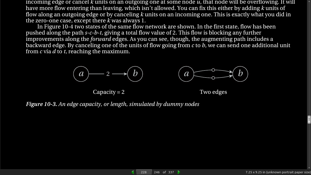
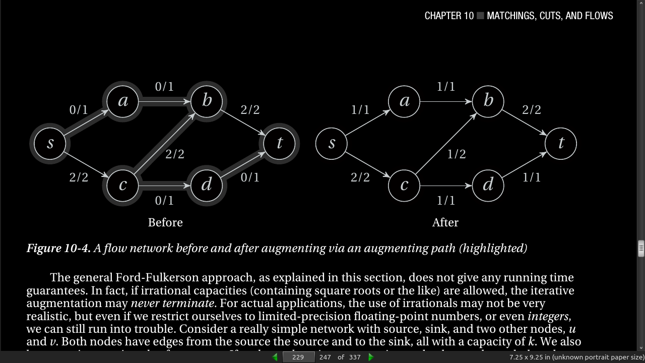
- Flow BACK is always zero, but flow can move “backwards” if there is forward flow that can be cancelled.
page 229:
page 230:
- Listing 10-3. Finding Augmenting Paths with BFS and Labeling
from collections import deque
inf = float('inf')

def bfs_aug(G, H, s, t, f):
  P, Q, F = {s: None}, deque([s]), {s: inf} # Tree, queue, flow label
  def label(inc):                           # Flow increase at v from u?
    if v in P or inc <= 0: return           # Seen? Unreachable? Ignore
    F[v], P[v] = min(F[u], inc), u          # Max flow here? From where?
    Q.append(v)                             # Discovered -- visit later
  while Q:                                  # Discovered, unvisited
    u = Q.popleft()                         # Get one (FIFO)
    if u == t: return P, F[t]               # Reached t? Augmenting path!
    for v in G[u]: label(G[u][v]-f[u,v])    # Label along out-edges
    for v in H[u]: label(f[v,u])            # Label along in-edges
  return None, 0                            # No augmenting path found
- Listing 10-4. The Ford-Fulkerson Method (by Default, the Edmonds-Karp Algorithm)
def ford_fulkerson(G, s, t, aug=bfs_aug): # Max flow from s to t
  H, f = tr(G), defaultdict(int)          # Transpose and flow
  while True:                             # While we can improve things
    P, c = aug(G, H, s, t, f)             # Aug. path and capacity/slack
    if c == 0: return f                   # No augm. path found? Done!
    u = t                                 # Start augmentation
    while u != s:                         # Backtrack to s
      u, v = P[u], u                      # Shift one step
      if v in G[u]: f[u,v] += c           # Forward edge? Add slack
      else: f[v,u] -= c                   # Backward edge? Cancel slack
page 231:
- Minimum cuts have several applications that don’t really look like max-flow problems. Consider, for example, the problem of allocating processes to two processors in a manner that minimizes the communication between them. Let’s say one of the processors is a GPU and that the processes have different running times on the two processors. Some fit the CPU better, while some should be run on the GPU. However, there might be cases where one fits on the CPU and one on the GPU, but where the two communicate extensively with each other. In that case, we might want to put them on the same processor, just to reduce the communication costs. How would we solve this? We could set up an undirected flow network with the CPU as the source and the GPU as the sink, for example. Each process would have an edge to both source and sink, with a capacity equal to the time it would take to run on that processor. We also add edges between processes that communicate, with capacities representing the communication overhead (in extra computation time) of having them on separate processors. The minimum cut would then distribute the processes on the two processors in such a way that the total cost is as small as possible—a nontrivial task if we couldn’t reduce to the min-cut problem.
page 234:
- Listing 10-5. The Busacker-Gowen Algorithm, Using Bellman-Ford for Augmentation
def busacker_gowen(G, W, s, t):            # Min-cost max-flow
  def sp_aug(G, H, s, t, f):               # Shortest path (Bellman-Ford)
    D, P, F = {s:0}, {s:None}, {s:inf,t:0} # Dist, preds and flow
    def label(inc, cst):                   # Label + relax, really
      if inc <= 0: return False            # No flow increase? Skip it
      d = D.get(u,inf) + cst               # New possible aug. distance
      if d >= D.get(v,inf): return False   # No improvement? Skip it
      D[v], P[v] = d, u                    # Update dist and pred
      F[v] = min(F[u], inc)                # Update flow label
      return True                          # We changed things!
    for rnd in G:                          # n = len(G) rounds
      changed = False                      # No changes in round so far
      for u in G:                          # Every from-node
        for v in G[u]:                     # Every forward to-node
          changed |= label(G[u][v]-f[u,v], W[u,v])
        for v in H[u]:                     # Every backward to-node
          changed |= label(f[v,u], -W[v,u])
      if not changed: break                # No change in round: Done
      else:                                # Not done before round n?
        raise ValueError('negative cycle') # Negative cycle detected
    return P, F[t]                         # Preds and flow reaching t
  return ford_fulkerson(G, s, t, sp_aug)   # Max-flow with Bellman-Ford
page 237:
- This chapter deals with a single core problem, finding maximum flows in flow networks, as well as specialized versions, such as maximum bipartite matching and finding edge-disjoint paths. You also saw how the minimum cut problem is the dual of the maximum flow problem, giving us two solutions for the price of one. Solving the minimum cost flow problem is also a close relative
· Chapter 11: Hard Problems and (Limited) Sloppiness
page 242:
-
Let’s say you’ve come to a small town where one of the main attractions is a pair of twin mountain peaks. The locals have affectionately called the two Castor and Pollux, after the twin brothers from Greek and Roman mythology. It is rumored that there’s a long-forgotten gold mine on the top of Pollux, but many an adventurer has been lost to the treacherous mountain. In fact, so many unsuccessful attempts have been made to reach the gold mine that the locals have come to believe it can’t be done. You decide to go for a walk and take a look for yourself.
-
After stocking up on donuts and coffee at a local roadhouse, you set off. After a relatively short walk, you get to a vantage point where you can see the mountains relatively clearly. From where you’re standing, you can see that Pollux looks like a really hellish climb—steep faces, deep ravines, and thorny brush all around it. Castor, on the other hand, looks like a climber’s dream. The sides slope gently, and it seems there are lots of handholds all the way to the top. You can’t be sure, but it seems like it might be a nice climb. Too bad the gold mine isn’t up there.
-
You decide to take a closer look, and pull out your binoculars. That’s when you spot something odd. There seems to be a small tower on top of Castor, with a zip line down to the peak of Pollux. Immediately, you give up any plans you had to climb Castor. Why? (If you don’t immediately see it, it might be worth pondering for a bit.)1
-
Of course, we’ve seen the exact situation before, in the discussions of hardness in Chapters 4 and 6. The zip line makes it easy to get from Castor to Pollux, so if Castor were easy, someone would have found the gold mine already.2 It’s a simple contrapositive: if Castor were easy, Pollux would be too; Pollux is not easy, so Castor can’t be either. This is exactly what we do when we want to prove that a problem (Castor) is hard. We take something we know is hard (Pollux) and show that it’s easy to solve this hard problem using our new, unknown one (we uncover a zip line from Castor to Pollux).
-
As I’ve mentioned before, this isn’t so confusing in itself. It can be easy to confuse things when we start talking about it in terms of reductions, though. For example, is it obvious to you that we’re reducing Pollux to Castor here? The reduction is the zip line, which lets us use a solution to Castor as if it were a solution to Pollux. In other words, if you want to prove that problem X is hard, find some hard problem Y and reduce it to X.
-
Caution The zip line goes in the opposite direction of the reduction. It’s crucial that you don’t get this mixed up, or the whole idea falls apart. The term reduction here means basically “Oh, that’s easy, you just …” In other words, if you reduce A to B, you’re saying “You want to solve A? That’s easy, you just solve B.” Or in this case: “You want to scale Pollux? That’s easy, just scale Castor (and take the zip line).” In other words, we’ve reduced the scaling of Pollux to the scaling of Castor (and not the other way around).
-
Hard Problems:
-
The problem is intractable—any algorithm solving it must be exponential.
-
We don’t know whether the problem is intractable, but no one has ever been able to find a polynomial algorithm for it.

page 256:
- I have talked about bipartite graphs several times already—graphs whose nodes can be partitioned into two sets so that all edges are between the sets (that is, no edges connect nodes in the same set). Another way of viewing this is as a two-coloring, where you color every node as either black or white (for example), but you ensure that no neighbors have the same color. If this is possible, the graph is bipartite.
page 261:
-
Some hard problems can be made easy or at least solvable it we allow ourselves to get sloppy. An approximation ratio is formed by the optimal solution and the and how good you can actually get.
-
Let’s consider the maximization case. If we know that the optimum will never be greater than A, and we know our approximation will never be smaller than B, we can be certain that the ratio of the two will never be greater than A/B.
page 262:
-
A Hamilton cycle connects all nodes, and the absolutely cheapest way of connecting all nodes is using a minimum spanning tree.
-
Listing 11-1. The “Twice Around the Tree” Algorithm, a 2-Approximation for Metric TSP
from collections import defaultdict # 2-approx for metric TSP
def mtsp(G, r):                     # Tree and cycle
  T, C = defaultdict(list), []      # Build a traversable MSP
  for c, p in prim(G, r).items():   # Child is parent's neighbor
    T[p].append(c)                  # Recursive DFS
  def walk(r):                      # Preorder node collection
    C.append(r)                     # Visit subtrees recursively
    for v in T[r]: walk(v)          # Traverse from the root
  walk(r)                           # At least half-optimal cycle
  return C
page 265:
- Note The nonlocal keyword, which is used in Listing 11-2, lets you modify a variable in a surrounding scope, just like global lets you modify the global scope. However, this feature is new in Python 3.0. If you want similar functionality in earlier Pythons, simply replace the initial sol = 0 by sol = [0], and later access the value using the expression sol[0] instead of just sol .
page 266:
- Listing 11-2. Solving the Knapsack Problem with the Branch and Bound Strategy
from __future__ import division
from heapq import heappush, heappop
from itertools import count

def bb_knapsack(w, v, c):
  sol = 0               # Solution so far
  n = len(w)            # Item count
  idxs = list(range(n))
  idxs.sort(key=lambda i: v[i]/w[i], reverse=True) # Sort by descending unit cost

  def bound(sw, sv, m):                     # Greedy knapsack bound
    if m == n: return sv                    # No more items?
    objs = ((v[i], w[i]) for i in idxs[m:]) # Descending unit cost order
    for av, aw in objs:                     # Added value and weight
      if sw + aw > c: break                 # Still room?
      sw += aw                              # Add wt to sum of wts
      sv += av                              # Add val to sum of vals
    return sv + (av/aw)*(c-sw)              # Add fraction of last item

  def node(sw, sv, m):                  # A node (generates children)
    nonlocal sol                        # "Global" inside bb_knapsack
    if sw > c: return                   # Weight sum too large? Done
    sol = max(sol, sv)                  # Otherwise: Update solution
    if m == n: return                   # No more objects? Return
    i = idxs[m]                         # Get the right index
    ch = [(sw, sv), (sw+w[i], sv+v[i])] # Children: without/with m
    for sw, sv in ch:                   # Try both possibilities
      b = bound(sw, sv, m+1)            # Bound for m+1 items
      if b > sol:                       # Is the branch promising?
        yield b, node(sw, sv, m+1)      # Yield child w/bound

  num = count()                       # Helps avoid heap collisions
  Q = [(0, next(num), node(0, 0, 0))] # Start with just the root
  while Q:                            # Any nodes left?
    _, _, r = heappop(Q)              # Get one
    for b, u in r:                    # Expand it ...
       heappush(Q, (b, next(num), u)) # ... and push the children
  return sol                          # Return the solution
page 271:
· PEDAL TO THE METAL: ACCELERATING PYTHON (Appendix A)
page 272:
-
GPULib and PyStream. These two packages let you use graphics processing units (GPUs) to accelerate your code. They don’t provide the kind of drop-in acceleration that a JIT compiler such as Psyco would, but if you have a powerful GPU, why not use it? Of the two projects, PyStream is older, and the efforts of Tech-X Corporation have shifted to the newer GPULib project. It gives you a high-level interface for various forms of numeric computation using GPUs.
-
Pyrex, Cython, and Shedskin. These three projects let you translate Python code into C or C++. Shedskin compiles plain Python code into C++, while Pyrex and Cython (which is a fork of Pyrex) primarily target C. In Cython (and Pyrex), you can add optional type declarations to your code, stating that a variable is (and will always be) an integer, for example. In Cython, there is also interoperability support for NumPy arrays, letting you write low-level code that accesses the array contents very efficiently. I have used this in my own code, achieving speedup factors of up to 300–400 for suitable code. The code that is generated by Pyrex and Cython can be compiled directly to an extension module that can be imported into Python.
-
SWIG, F2PY and Boost.Python. These tools let you wrap C/C++, Fortran, and C++ code, respectively. Although you could write your own wrapper code for accessing your extension modules, using a tool like one of these takes a lot of the tedium out of the job—and makes it more likely that the result will be correct. For example, when using SWIG, you run a command-line tool on your C (or C++) header files, and wrapper code is generated. A bonus to using SWIG is that it can generate wrappers for a lot of other languages, beside Python, so your extension could be available for Java or PHP as well, for example.
-
ctypes, llvm-py, and CorePy. These are modules that let you manipulate low-level code objects in your Python code. The ctypes module lets you build C objects in memory and call C functions in shared libraries (such as DLLs) with those objects as parameters. The llvm-py package gives you a Python API to the LLVM, mentioned earlier, which lets you build code and then compile it efficiently. If you wanted, you could use this to build your own compiler (perhaps for a language of your own?) in Python. CorePy also lets you manipulate and efficiently run code objects, although it works at the assembly level. (Note that ctypes is part of the Python standard library.)
page 273:
-
Weave, Cinpy, and PyInline. These three packages let you use C (or some other languages) directly in your Python code. This is done quite cleanly, by keeping the C code in multiline Python strings, which are then compiled on the fly. The resulting code object is then available to your Python code, using facilities such as ctypes for the interfacing.
-
Table A-1. URLs for Acceleration Tool Web Sites
· LIST OF PROBLEMS AND ALGORITHMS (Appendix B)
-
In most descriptions in this appendix, n refers to the problem size (such as the number of elements in a sequence). For the special case of graphs, though, n refers to the number of nodes, and m refers to the number of edges.
-
Cliques and independent sets. A clique is a graph where there is an edge between every pair of nodes. The main problem of interest here is finding a clique in a larger graph (that is, identifying a clique as a subgraph). An independent set in a graph is a set of nodes where no pair is connected by an edge. In other words, finding an independent set is equivalent to taking the complement of the edge set and finding a clique. Finding a k-clique (a clique of k nodes) or finding the largest clique in a graph (the max- clique problem) is NP-hard. (For more information, see Chapter 11.)
-
Closest pair. Given a set of points in the Euclidean plane, find the two points that are closest to each other. This can be solved in loglinear time using the divide-and-conquer strategy (see Chapter 6).
-
Compression and optimal decision trees. A Huffman tree is a tree whose leaves have weights (frequencies), and the sum of their weights multiplied by their depth is as small as possible. This makes such trees useful for constructing compression codes and as decision trees when a probability distribution is known for the outcomes. Huffman trees can be built using Huffman’s algorithm, described in Chapter 7 (Listing 7-1).
page 276:
-
Connected and strongly connected components. An undirected graph is connected if there is a path from every node to every other. A directed graph is connected if its underlying undirected graph is connected. A connected component is a maximal subgraph that is connected. Connected components can be found using traversal algorithms such as DFS (Listing 5-5) or BFS (Listing 5-9), for example. If there is a (directed) path from every node to every other in a directed graph, it is called strongly connected. A strongly connected component (SCC) is a maximal subgraph that is strongly connected. SCCs can be found using Kosaraju’s algorithm (Listing 5-10).
-
Convex hulls. A convex hull is the minimum convex region containing a set of points in the Euclidean plane. Convex hulls can be found in loglinear time using the divide-and-conquer strategy (see Chapter 6).
-
Finding the minimum/maximum/median. Finding the minimum and maximum of a sequence can be found in linear time by a simple scan. Repeatedly finding and extracting the maximum or minimum in constant time, given linear-time preparation, can be done using a binary heap. It is also possible to find the kth smallest element of a sequence (the median for k = n/2) in linear (or expected linear) time, using the select or randomized select. (For more information, see Chapter 6).
-
Flow and cut problems. How many units of flow can be pushed through a network with flow capacities on the edges? That is the max-flow problem. An equivalent problem is finding the set of edge capacities that most constrain the flow; this is the min-cut problem. There are several versions of these problems. For example, you could add costs to the edges, and find the cheapest of the maximum flows. You could add lower bound on each edge and look for a feasible flow. You could even add separate supplies and demands in each node. These problems are dealt with in detail in Chapter 10.
-
Graph coloring. Try to color the nodes of a graph so that no neighbors share a color. Now try to do this with a given number of colors, or even to find the lowest such number (the chromatic number of the graph). This is an NP-hard problem in general. If, however, you’re asked to see if a graph is two-colorable (or bipartite), the problem can be solved in linear time using simple traversal. The problem of finding a clique cover is equivalent to finding an independent set cover, which is an identical problem to graph coloring. (See Chapter 11 for more on graph coloring.)
-
Hamilton cycles/paths and TSP … and Euler tours. Several path and subgraph problems can be solved efficiently. If, however, you want to visit every node exactly once, you’re in trouble. Any problem involving this constraint is NP-hard, including finding a Hamilton cycle (visit every node once and return), a Hamilton path (visit every node once, without returning), or a shortest tour of a complete graph (the Traveling Salesman/Salesrep problem). The problems are NP-hard both for the directed and undirected case (see Chapter 11). The related problem of visiting every edge exactly once, though— finding a so-called Euler tour—is solvable in polynomial time (see Chapter 5). The TSP problem is NP- hard even for special cases such as using Euclidean distances in the plane, but it can be efficiently approximated to within a factor of 1.5 for this case, and for any other metric distance. Approximating the TSP problem in general, though, is NP-hard. (See Chapter 11 for more information.)
-
Longest increasing subsequence. Find the longest subsequence of a given sequence whose elements are in increasing order. This can be solved in loglinear time using dynamic programming (see Chapter 8).
-
Matching. There are many matching problems, all of which involve linking some object to others. The problems discussed in this book are bipartite matching and min-cost bipartite matching (Chapter 10) and the stable marriage problem (Chapter 7). Bipartite matching (or maximum bipartite matching) involves finding the greatest subset of edges in a bipartite graph so that no two edges in the subset share a node. The min-cost version does the same, but minimizes the sum of edge costs over this subset. The stable marriage problem is a bit different; there, all men and women have preference rankings of the members of the opposite sex. A stable set of marriages is characterized by the fact that you can’t find a pair that would rather have each other than their current mates.
page 277:
-
Minimum spanning trees. A spanning tree is a subgraph whose edges form a tree over all the nodes of the original graph. A minimum spanning tree is one that minimizes the sum of edge costs. Minimum spanning trees can be found using Kruskal’s algorithm (Listing 7-4) or Prim’s algorithm (Listing 7-5), for example. Because the number of edges is fixed, a maximum spanning tree can be found by simply negating the edge weights.
-
Partitioning and bin packing. Partitioning involves dividing a set of numbers into two sets with equal sums, while the bin packing problem involves packing a set of numbers into a set of “bins” so that the sum in each bin is below a certain limit and so that the number of bins is as small as possible. Both problems are NP-hard. (See Chapter 11.)
-
SAT, Circuit-SAT, k-CNF-SAT. These are all varieties of the satisfaction problem (SAT), which asks you to determine whether a given logical (Boolean) formula can ever be true, if you’re allowed to set the variables to whatever truth values you want. The circuit-SAT problem simply uses logical circuits rather than formulas, and k-CNF-SAT involves formulas in conjunctive normal form, where each clause consists of k literals. The latter can be solved in polynomial time for k = 2. The other problems, as well as k-CNF-SAT for k > 2, are NP-complete. (See Chapter 11.)
-
Searching. This is a very common and extremely important problem. You have a key and want to find an associated value. This is, for example, how variables work in dynamic languages such as Python. It’s also how you find almost anything on the Internet these days. Two important solutions are hash tables (see Chapter 2) and binary search or search trees (see Chapter 6). Given a probability distribution for the objects in the data set, optimal search trees can be constructed using dynamic programming (see Chapter 8).
-
Sequence comparison. You may want to compare two sequences to know how similar (or dissimilar) they are. One way of doing this is to find the longest subsequence the two have in common (longest common subsequence) or to find the minimum number of basic edit operations to go from one sequence to the other (so-called edit distance, or Levenshtein distance). These two problems are more or less equivalent; see Chapter 8 for more information.
-
Sequence modification. Inserting an element into the middle of a linked list is cheap (constant time), but finding a given location is costly (linear time); for an array, the opposite is true (constant lookup, linear insert, because all later elements must be shifted). Appending can be done cheaply for both structures, though (see the black box sidebar on list in Chapter 2).
-
Set and vertex covers. A vertex cover is a set of vertices that cover (that is, are adjacent to) all the edges of the graph. A set cover is a generalization of this idea, where the nodes are replaced with subsets, and you want to cover the entire set. The problem lies in constraining or minimizing the number of nodes/subsets. Both problems are NP-hard (see Chapter 11).
-
Shortest paths. This problem involves finding the shortest path from one node to another, from one node to all the others (or vice versa), or from all nodes to all others. The one-to-one, one-to-all, and all- to-one cases are solved the same way, normally using BFS for unweighted graphs, DAG shortest path for DAGs, Dijkstra’s algorithm for nonnegative edge weights, and Bellman–Ford in the general case. To speed up things in practice (although without affecting the worst-case running time), one can also use bidirectional Dijkstra, or the A* algorithm. For the all pairs shortest paths problem, the algorithms of choice are probably Floyd–Warshall or (for sparse graphs) Johnson’s algorithm. If the edges are nonnegative, Johnson’s algorithm is (asymptotically) equivalent to running Dijkstra’s algorithm from every node (which may be more effective). (For more information on shortest path algorithms, see Chapters 5 and 9.) Note that the longest path problem (for general graphs) can be used to find Hamilton paths, which means that it is NP-hard. This, in fact, means that the shortest path problem is also NP- hard in the general case. If we disallow negative cycles in the graph, however, our polynomial algorithms will work.
page 278:
-
Sorting and element uniqueness. Sorting is an important operation and an essential subroutine for several other algorithms. In Python, you would normally sort by using the list.sort method or the sorted function, both of which use a highly efficient implementation of the timsort algorithm. Other algorithms include insertion sort, selection sort, and gnome sort (all of which have a quadratic running time), as well as heapsort, mergesort, and quicksort (which are loglinear, although this holds only in the average case for quicksort). For the info on the quadratic sorting algorithms, see Chapter 5; for the loglinear (divide-and-conquer) algorithms, see Chapter 6. Deciding whether a set of real numbers contains duplicates cannot (in the worst case) be solved with a running time better than loglinear. By reduction, neither can sorting.
-
The halting problem. Determine whether a given algorithm will terminate with a given input. The problem is undecidable (that is, unsolvable) in the general case (see Chapter 11).
-
The knapsack problem and integer programming. The knapsack problem involves choosing a valuable subset of a set of items, under certain constraints. In the (bounded) fractional case, you have a certain amount of some substances, each of which has a unit value (value per unit of weight). You also have a knapsack that can carry a certain maximum weight. The (greedy) solution is to take as much as you can of each substance, starting with the one with the highest unit value. For the integral knapsack problem, you can only take entire items—fractions aren’t allowed. Each item has a weight and a value. For the bounded case (also known as 0-1 knapsack) you have a limited number of objects of each type. (Another perspective would be that you have a fixed set of objects that you either take or not.) In the unbounded case, you can take as many as you want from each of a set of object types (still respecting your carrying capacity, of course). A special case known as the subset sum problem involves selecting a subset of a set of numbers so that the subset has a given sum. These problems are all NP-hard (see Chapter 11), but admit pseudopolynomial solutions based on dynamic programming (see Chapter 8). The fractional knapsack case, as explained, can even be solved in polynomial time using a greedy strategy (see Chapter 7). Integer programming is, in some ways, a generalization of the knapsack problem (and is therefore obviously NP-hard). It is simply linear programming where the variables are constrained to be integers.
-
Topological sorting. Order the nodes of a DAG so that all the edges point in the same direction. If the edges represent dependencies, a topological sorting represents an ordering that respects the dependencies. This problem can be solved by a form of reference counting (see Chapter 4) or by using DFS (see Chapter 5).
-
Traversal. The problem here is to visit all the objects in some connected structure, usually represented as nodes in a graph or tree. The idea can be either to visit every node or to visit only those needed to solve some problem. The latter strategy of ignoring parts of the graph or tree is called pruning and is used (for example) in search trees and in the branch and bound strategy. For a lot on traversal, see Chapter 5.
· ALGORITHMS AND DATA STRUCTURES (Appendix B)
-
2-3-trees. Balanced tree structure, allowing insertions, deletions, and search in worst-case Θ(lg n) time. Internal nodes can have two or three children, and the tree is balanced during insertion by splitting nodes, as needed. (See Chapter 6.)
-
A*. Heuristically guided single source shortest path algorithm. Suitable for large search spaces. Instead of choosing the node with the lowest distance estimate (as in Dijkstra’s), the node with the lowest heuristic value (sum of distance estimate and guess for remaining distance) is used. Worst-case running time identical to Dijkstra’s algorithm. (See Listing 9-10.)
-
AA-tree. 2-3-trees simulated using node rotations in a binary tree with level-numbered nodes. Worst- case running times of Θ(lg n) for insertions, deletions, and search. (See Listing 6-6.)
-
Bellman–Ford. Shortest path from one node to all others in weighted graphs. Looks for a shortcut along every edge n times. Without negative cycles, correct answer guaranteed after n –1 iterations. If there’s improvement in the last round, a negative cycle is detected, and the algorithm gives up. Running time Θ(nm). (See Listing 9-2.)
-
Bidirectional Dijkstra. Dijkstra’s algorithm run from start and end node simultaneous, with alternating iterations going to each of the two algorithms. The shortest path is found when the two meet up in the middle (although some care must be taken at this point). The worst-case running time is just like for Dijkstra’s algorithm. (See Listings 9-8 and 9-9.)
-
Binary search trees. A binary tree structure where each node has a key (and usually an associated value). Descendant keys are partitioned by the node key: smaller keys go in the left subtree, and greater keys go in the right. On the average, the depth of any node is logarithmic, giving an expected insertion and search time of Θ(lg n). Without extra balancing, though (such as in the AA-tree), the tree can become unbalanced, giving linear running times. (See Listing 6-2.)
-
Bisection, binary search. A search procedure that works in a manner similar to search trees, by repeated halving the interval of interest in a sorted sequence. The halving is performed by inspecting the middle element, and deciding whether the sought value must lie to the left or right. Running time Θ(lg n). A very efficient implementation can be found in the bisect module. (See Chapter 6.)
-
Branch and bound. A general algorithmic design approach. Searches a space of solutions in a depth-first or best-first order by building and evaluating partial solutions. A conservative estimate is kept for the optimal value, while an optimistic estimate is computed for a partial solution. If the optimistic estimate is worse than the conservative one, the partial solution is not extended, and the algorithm backtracks. Often used to solve NP-hard problems. (See Listing 11-2 for a branch-and-bound solution to the 0-1 knapsack problem.)
-
Breadth-First Search (BFS). Traversing a graph (possibly a tree) level by level, thereby also identifying (unweighted) shortest path. Implemented by using a FIFO queue to keep track of discovered nodes. Running time Θ(n + m). (See Listing 5-9.)
-
Bucket sort. Sort numerical values that are evenly (uniformly) distributed in a given interval by dividing the interval into n equal-sized buckets and placing the values in them. Expected bucket size is constant, so they can be sorted with (for example) insertion sort. Total running time Θ(n). (See Chapter 4.)
-
Busacker–Gowen. Finds the cheapest max-flow (or the cheapest flow with a given flow value) in a network by using the cheapest augmenting paths in the Ford–Fulkerson approach. These paths are found using Bellman–Ford or (with some weight adjustments) Dijkstra’s algorithm. The running time in general depends on the maximum flow value and so is pseudopolynomial. For a maximum flow of k, the running time is (assuming Dijkstra’s algorithm is used) O(km lg n). (See Listing 10-5.)
page 280:
-
Christofides’ algorithm. An approximation algorithm (with an approximation ratio bound of 1.5) for the metric TSP problem. Finds a minimum spanning tree and then a minimum matching2 among the odd- degree nodes of the tree, short-circuiting as needed to make a valid tour of the graph. (See Chapter 11.)
-
Counting sort. Sort integers with a small value range (with at most Θ(n) contiguous values) in Θ(n) time. Works by counting occurrences and using the cumulative counts to directly place the numbers in the result, updating the counts as it goes. (See Chapter 4.)
-
DAG Shortest Path. Finds the shortest path from one node to all others in a DAG. Works by finding a topological sorting of the nodes and then relaxing all out-edges (or, alternatively, all in-edges) at every node from left to right. Can (because of the lack of cycles) also be used to find longest paths. Running time Θ(n + m). (See Listing 8-4.)
-
Depth-First Search (DFS). Traversing a graph (possibly a tree) by going in depth and then backtracking. Implemented by using a LIFO queue to keep track of discovered nodes. By keeping track of discover- and finish-times, DFS can also be used as a subroutine in other algorithms (such as topological sorting or Kosaraju’s algorithm). Running time Θ(n + m). (See Listings 5-4, 5-5, and 5-6.)
-
Dijkstra’s algorithm. Find the shortest paths from one node to all others in a weighted graph, as long as there are no negative edge weights. Traverses the graph, repeatedly selecting the next node using a priority queue (a heap). The priority is the current distance estimate of the node. These estimates are updated whenever a shortcut is found from a visited node. The running time is Θ((m+n) lg n), which is simply Θ(m lg n) if the graph is connected.
-
Double-ended queues. FIFO queues implemented using linked lists (or linked lists of arrays), so that inserting and extracting objects at either end can be done in constant time. An efficient implementation can be found in the collections.deque class. (See Chapter 5.)
-
Dynamic arrays, vectors. The idea of having extra capacity in an array, so appending is efficient. By relocating the contents to a bigger array, growing it by a constant factor, when it fills up, appends can be constant in average (amortized) time. (See Chapter 2.)
-
Edmonds–Karp. The concrete instantiation of the Floyd–Warshall method where traversal is performed using BFS. Finds min-cost flow in Θ(nm2) time. (See Listing 10-4.)
-
Floyd–Warshall. Finds shortest paths from each nodes to all others. In iteration k, only the first k nodes (in some ordering) are allowed as intermediate nodes along the paths. Extending from k –1 involves checking whether the shortest paths to and from k via the first k –1 nodes is shorter than simply going directly via these nodes. (That is, node k is either used or not, for every shortest path.) Running time is Θ(n3). (See Listing 9-6.)
-
Ford–Fulkerson. A general approach to solving max-flow problems. The method involves repeatedly traversing the graph to find a so-called augmenting path, a path along which the flow can be increased (augmented). The flow can be increased along an edge if it has extra capacity, or it can be increased backward across an edge (that is, canceled) if there is flow along the edge. Thus, the traversal can move both forward and backward along the directed edges, depending on the flow across them. The running time depends on the traversal strategy used. (See Listing 10-4.)
-
Gale–Shapley. Finds a stable set of marriages given preference rankings for a set of men and women. Any unengaged men propose to the most preferred woman they haven’t proposed to. Each woman will choose her favorite among her current suitors (possibly staying with her fiancé). Can be implemented with quadratic running time. (See Chapter 7.)
page 281:
-
Gnome sort. A simple sorting algorithm with quadratic running time. Probably not an algorithm you’ll use in practice. (See Listing 3-1.)
-
Hashing, hash tables. Look up a key to get the corresponding value, just like in a search tree. Entries are stored in an array, and their positions are found by computing a (pseudorandom, sort of) hash value of the key. Given a good hash function and enough room in the array, the expected running time of insertion, deletion and lookup is Θ(1). (See Chapter 2.)
-
Heaps, heapsort. Heaps are efficient priority queues. With linear-time preprocessing, a min- (max-) heap will let you find the smallest (largest) element in constant time and extract or replace it in logarithmic time. Adding an element can also be done in logarithmic time. Conceptually, a heap is a full binary tree where each node is smaller (larger) than its children. When modifications are made, this property can be repaired with Θ(lg n) operations. In practice, heaps are usually implemented using arrays (with nodes encoded as array entries). A very efficient implementation can be found in the heapq module. Heapsort is like selection sort, except that the unsorted region is a heap, so finding the largest element n times gives a total running time of Θ(n lg n). (See Chapter 6.)
-
Huffman’s algorithm. Builds Huffman trees, which can be used for building optimal prefix codes, for example. Initially, each element (for example, character in an alphabet) is made into a single-node tree, with a weight equal to its frequency. In each iteration, the two lightest trees are picked, combining them with a new root, giving the new tree a weight equal to the sum of the original two tree weights. This can be done in loglinear time (or, in fact, in linear time if the frequencies are presorted). (See Listing 7-1.)
-
Insertion sort. A simple sorting algorithm with quadratic running time. It works by repeatedly inserting the next unsorted element in an initial sorted segment of the array. For small data sets, it can actually be preferable to more advanced (and optimal) algorithms such as merge sort or quicksort. (In Python, though, you should use list.sort or sorted if at all possible.) (See Listing 4-3.)
-
Interpolation search. Similar to ordinary binary search, but linear interpolation between the interval endpoints is used to guess the correct position, rather than simply looking at the middle element. The worst-case running time is still Θ(lg n), but the average-case running time is O(lg lg n) for uniformly distributed data. (Mentioned in the “If You’re Curious …” section of Chapter 6.)
-
Iterative deepening DFS. Repeated runs of DFS, where each run has a limit to how far it can traverse. For structures with some fanout, the running time will be the same as for DFS or BFS (that is, Θ(n + m)). The point is that it has the advantages of BFS (it finds shortest paths, and explores large state spaces conservatively), with the smaller memory footprint of DFS. (See Listing 5-8.)
-
Johnson’s algorithm. Finds shortest paths from every node to all others. Basically runs Dijkstra’s from every node. However, it uses a trick so that it also works with negative edge weights: it first runs Bellman–Ford from a new start node (with added edges to all existing nodes) and then uses the resulting distances to modify the edge weights of the graph. The modified weights are all nonnegative but are set so that the shortest paths in the original graph will also be the shortest paths in the modified graph. Running time Θ(mn lg n). (See Listing 9-4.)
-
Kosaraju’s algorithm. Finds strongly connected components, using DFS. First, nodes are ordered by their finish times. Then the edges are reversed, and another DFS is run, selecting start nodes using the first ordering. Running time Θ(n + m). (See Listing 5-10.)
page 282:
-
Kruskal’s algorithm. Finds a minimum spanning tree by repeatedly adding the smallest remaining edge that doesn’t create a cycle. This cycle checking can (with some cleverness) be performed very efficiently, so the running time is dominated by sorting the edges. All in all, the running time is Θ(m lg n). (See Chapter 7.)
-
Linked lists. An alternative to arrays for representing sequences. Although linked lists are cheap (constant time) to modify once you’ve found the right entries, finding those normally takes linear time. Linked lists are implemented sort of like a path, with each node pointing to the next. Note that Python’s list type is implemented as an array, not a linked list. (See Chapter 2.)
-
Merge sort. The archetypal divide-and-conquer algorithm. It divides the sequence to be sorted in the middle, sorts the two halves recursively, and then merges the two sorted halves in linear time. The total running time is Θ(n lg n). (See Listing 6-5.)
-
Ore’s algorithm. An algorithm for traversing actual mazes in person, by marking passage entries and exits. In many ways similar to iterative deepening DFS or BFS. (See Chapter 5.)
-
Prim’s algorithm. Grows a minimum spanning tree by repeatedly adding the node closest to the tree. It is, at core, a traversal algorithm, and uses a priority queue, just like Dijkstra’s algorithm. (See Listing 7-5.)
-
Radix sort. Sorts numbers (or other sequences) by digit (element), start with the least significant one. As long as the number of digits is constant, and the digits can be sorted in linear time (using, for example, counting sort), the total running time is linear. It’s important that the sorting algorithm used on the digits is stable. (See Chapter 4.)
-
Randomized Select. Finds the median, or, in general, the kth order statistik (the kth smallest element). Works sort of like “half a quicksort.” It chooses a pivot element at random (or arbitrarily), and partitions the other elements to the left (smaller elements) or right (greater elements) of the pivot. The search then continues in the right portion, more or less like binary search. Perfect bisection is not guaranteed, but the expected running time is still linear. (See Listing 6-3.)
-
Select. The rather unrealistic, but guaranteed linear, sibling of randomized select. It works as follows: Divide the sequence into groups of five. Find the median in each using insertion sort. Find the median of these medians recursively, using select. Use this median of medians as a pivot, and partition the elements. Now run select on the proper half. In other words, it’s very similar to randomized select—the difference is that it can guarantee that a certain percentage will end up on either side of the pivot, avoiding the totally unbalanced case. Not really an algorithm you’re likely to use in practice, but it’s important to know about. (See Chapter 6.)
-
Selection sort. A simple sorting algorithm with quadratic running time. Very similar to insertion sort, but instead of repeatedly inserting the next element into the sorted section, you repeatedly find (that is, select) the largest element in the unsorted region (and swap it with the last unsorted element). (See Listing 4-5.)
-
Timsort. A super-duper in-place sorting algorithm based on mergesort. Without any explicit conditions for handling special cases, it is able to take into account partially sorted sequences, including segments that are sorted in reverse, and can therefore sort many real-world sequences faster than what would seem possible. The implementation in list.sort and sorted is also really fast, so if you need to sort something, that’s what you should use. (See Chapter 6.)
-
Topological sorting by reference counting. Orders the nodes of a DAG so that all edges go from left to right. This is done by counting the number of in-edges at each node. The nodes with an in-degree of zero are kept in a queue (could just be a set; the order doesn’t matter). Nodes are taken from the queue and placed in the topological sorted order. As you do so, you decrement the counts for the nodes that this node has edges to. If any of them reaches zero, they are placed in the queue. (See Listing 4-11.)
page 283:
-
Topological sorting with DFS. Another algorithm for sorting DAG nodes topologically. The idea is simple: perform a DFS and sort the nodes by inverse finish time. To easily get a linear running time, you can instead simply append nodes to your ordering as they receive their finish times in DFS. (See Listing 5-7.)
-
Tremaux’s algorithm. Like Ore’s algorithm, this is designed to be executed in person, while walking through a maze. The pattern traced by a person executing Tremaux’s algorithm is essentially the same as that of DFS. (See Chapter 5.)
-
Twice around the tree. An approximation algorithm for the metric TSP problem, guaranteed to yield a solution with a cost of at most twice the optimum. First, it builds a minimum spanning tree (which is less than the optimum), and then it “walks around” the tree, taking shortcuts to avoid visiting the same edge twice. Because of the metricity, this is guaranteed to be cheaper than walking each edge twice. This last traversal can be implemented by a preorder DFS. (See Listing 11-1.)
· GRAPH TERMINOLOGY (Appendix C)
page 286:
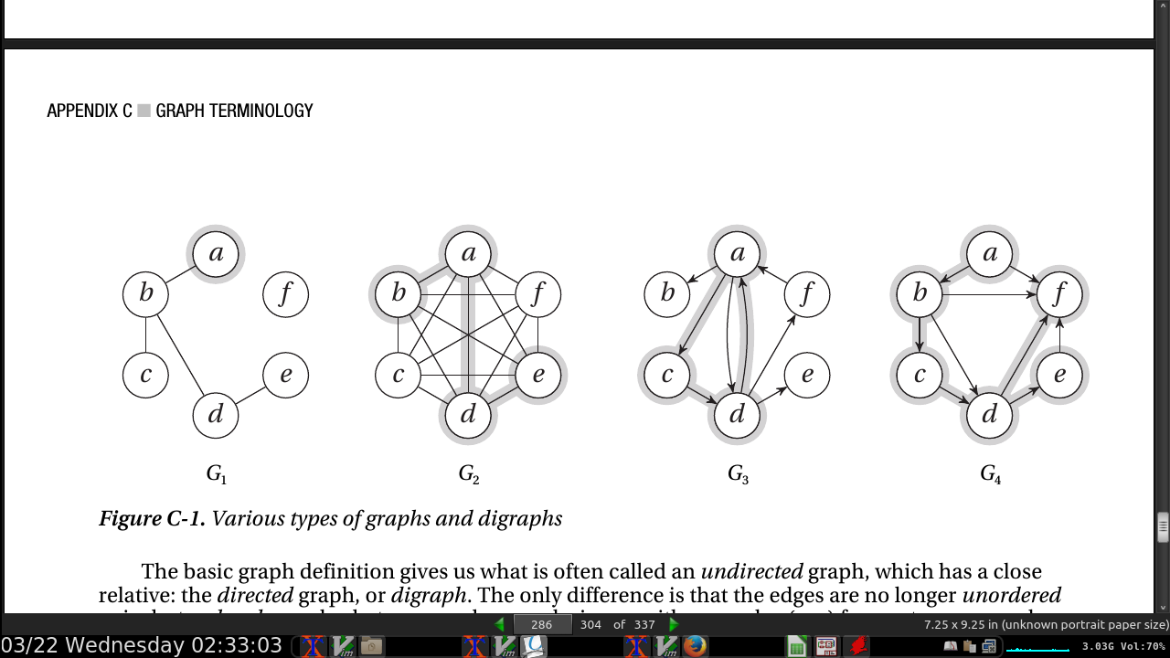
page 288:
-
Another term for an undirected, acyclic graph is forest, and the connected components of a forest are called trees. In other words, a tree is a connected forest (that is, a forest consisting of a single connected component). For example, G1 is a forest with two trees. In a tree, nodes with a degree of one are called leaves (or external nodes),4 while all others are called internal nodes. The larger tree in G1, for example, has three leaves and two internal nodes. The smaller tree consists of only an internal node, although talking about leaves and internal nodes may not make much sense with fewer than three nodes.
-
Trees have several interesting and important properties, some of which are dealt with in relation to specific topics throughout the book. I’ll give you a few right here, though. Let T be an undirected graph with n nodes. Then the following statements are equivalent (Exercise 2-9 asks you to show that this is, indeed, the case):
- T is a tree (that is, it is acyclic and connected).
- T is acyclic, and has n –1 edges.
- T is connected, and has n –1 edges.
- Any two nodes are connected by exactly one path.
- T is acyclic, but adding any new edge to it will create a cycle.
- T is connected, but removing any edge yields two connected components.
- In other words, any one of these statements of T, on its own, characterizes it as well as any of the others. If someone tells you that there is exactly one path between any pair of nodes in T, for example, you immediately know that it is connected and has n –1 edges and that it has no cycles. Quite often, we anchor our tree by choosing a root node (or simply root). The result is called a rooted tree, as opposed to the free trees we’ve been looking at so far. (If it is clear from the context whether a tree has a root or not, I will simply use the unqualified term tree in both the rooted and free case.) Singling out a node like this lets us define the notions of up and down. Paradoxically, computer scientists (and graph theorists in general) tend to place the root at the top and the leaves at the bottom. (We probably should get out more …). For any node, up is in the direction of the root (along the single path between the node and the root). Down is then any other direction (automatically in the direction of the leaves). Note that in a rooted tree, the root is considered an internal node, not a leaf, even if it happens to have a degree of one.