Home · Book Reports · 2016 · O'reilly Graph Databases
- Author :: Ian Robinson, Jim Webber, and Emil Eifrem
- Publication Year :: 2013
- Read Date :: 2016-09-27
- Source :: OREILLY-GRAPH_DATABASES.pdf
designates my notes. / designates important.
Thoughts
Easy to understand introduction to graph databases. Neo4j is, so far, useful and intuitive. In the little I’ve used neo4j (about a week fiddling around with it) it seems very straight forward to use with cypher and py2neo.
I have been wanting to try MongoDB for a while, and this book made me want to look at the newer database options more than ever. Cassandra also looked appealing.
The mapping structure does emulate how I think. The connections or relationships are intuitive. While working on CONected I was able to sketch a few ideas, each covering a particular domain, and then amalgamate them together in one graph. It is too early to tell how well it will work, but it was quick to develop and, again, is intuitively linked to the real world.
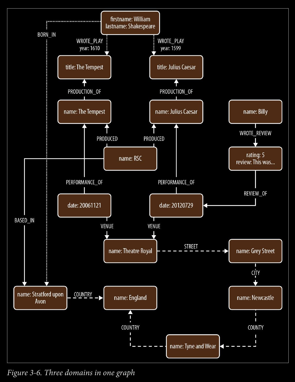
The Shakespeare example, with 3 overlapping domains, is great. In developing a graph for CONected, it seems like I'll want to model people in an organization, then multiple of these organizational subgraphs into a larger national and global graphs. A similar model can be constructed of government departments inside national governments inside global governments. Something json-like:{"World Gov":
{"Nato": {"USA Gov": {"CIA":["Alice", "Bob", "Charlie"],
"Whitehouse":["George", "George", "Bill"],
"TV":["Lies", "About", "Fantasies"]},
"English Gov": {"Parliament":["Tony", "Margaret"],
"Monty Python": ["Holy Grail"],
"Tea": ["Black", "Green"]}
}
}
{"EU": ["..."] }
"Japanese Gov": {"Whales": ["Sushi", "Dinner"],
"Anime": ["Luffy", "Chopper"],
"Sexbots": ["Beep", "Boop", "Ooh"]}
}
CHAPTER 1 - Introduction:
Page 9:
-
Graphs are naturally additive, meaning we can add new kinds of relationships, new nodes, and new subgraphs to an existing structure without disturbing existing queries and application functionality.
-
Because of the graph model’s flexibility, we don’t have to model our domain in exhaustive detail ahead of time
-
Schema-free
CHAPTER 2 - Options for Storing Connected Data:
page 12:
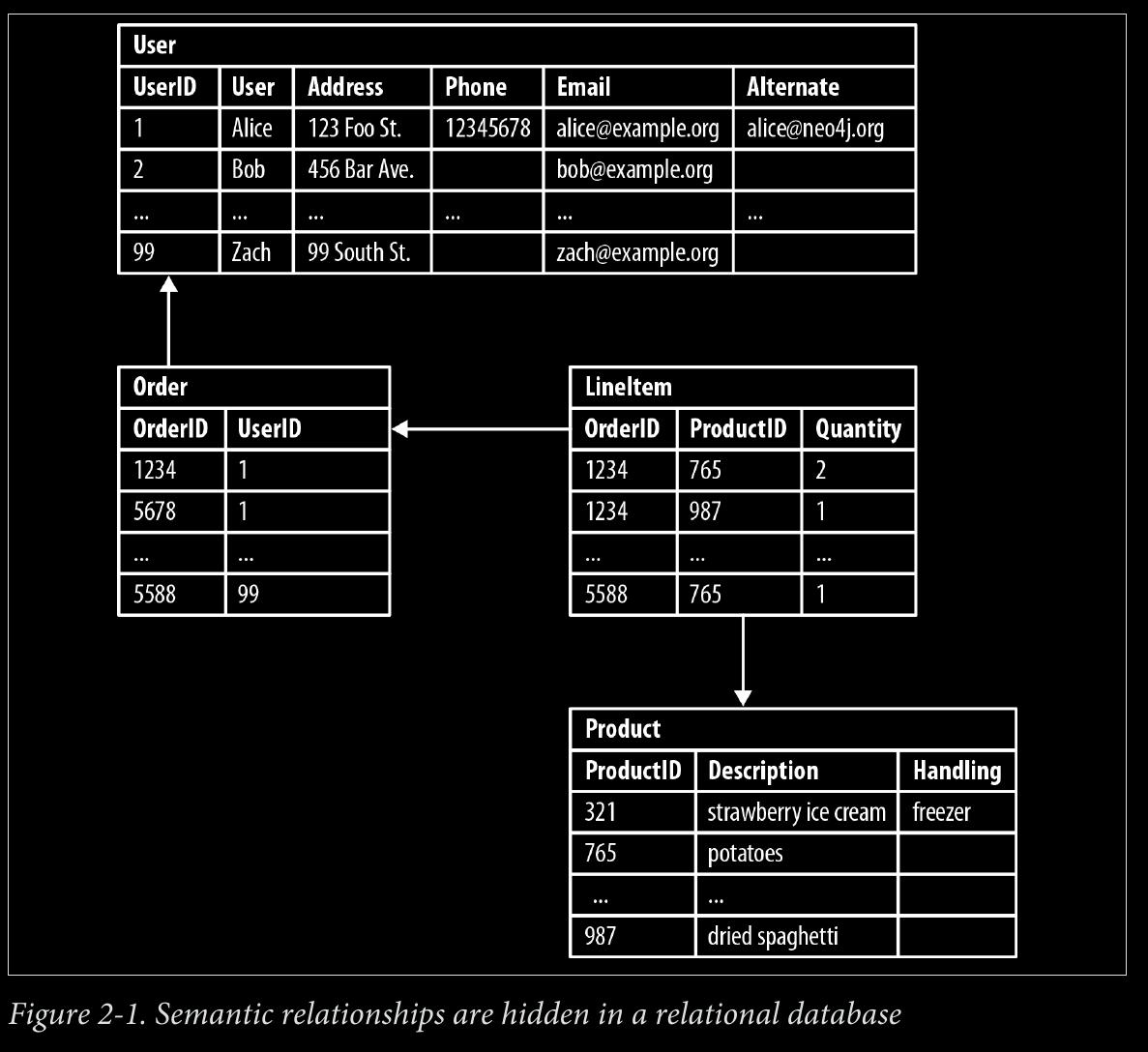
- Join tables add accidental complexity; they mix business data with foreign key metadata.
page 17:
- O(n) is considered too slow. O(log n) is “expected”.
page 18:
- The previous examples have dealt with implicitly connected data. As users we infer semantic dependencies between entities, but the data models—and the databases them‐ selves—are blind to these connections.

CHAPTER 3 - Data Modeling with Graphs:
page 25:
- All models are abstractions, but graph models “fit” real-world thinking
page 27:
- Cypher is arguably the easiest graph query language to learn, and is a great basis for learning about graphs. Once you understand Cypher, it becomes very easy to branch out and learn other graph query languages.
page 28:
- A Cypher query anchors one or more parts of a pattern to specific starting locations in a graph, and then flexes the unanchored parts around to find local matches.
page 29:
- The starting locations—the anchor points in the real graph, to which some parts of the pattern are bound—are discovered in one of two ways. The most common method is to use an index. Neo4j uses indexes as naming services; that is, as ways of finding starting locations based on one or more indexed property values.
page 37:
-
Relational databases—with their rigid schemas and complex modeling characteristics—are not an especially good tool for supporting rapid change.
-
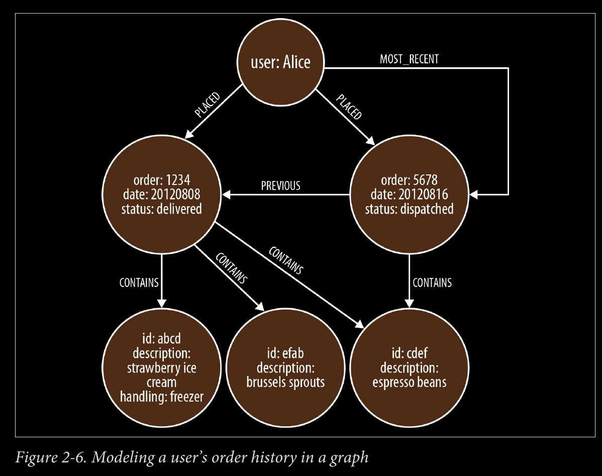
Instead of transforming a domain model’s graph-like representation into tables, we enrich it
-
domain modeling is completely isomorphic to graph modeling.
-
in a graph database what you sketch on the whiteboard is typically what you store in the database.
page 39:
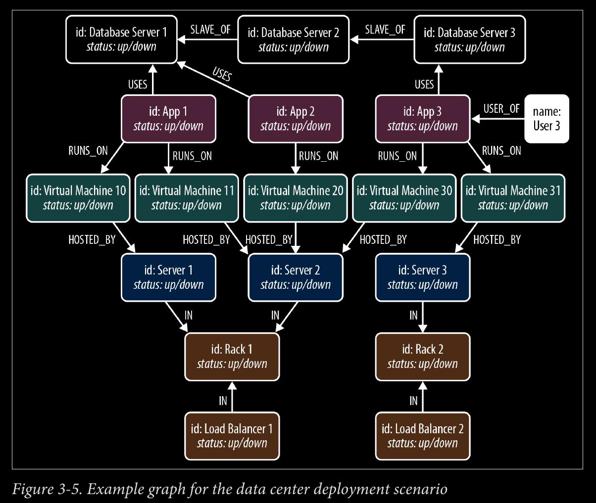
- adopt a design for query-ability mindset. To validate that the graph supports the kinds of queries we expect to run on it, we must describe those queries. example graph page 38.
START user=node:users(name = 'User 3')
MATCH (user)-[*1..5]-(asset)
WHERE asset.status! = 'down'
RETURN DISTINCT asset
page 40:
- starting from the user who reported the problem, we MATCH against all assets in the graph along an undirected path of length 1 to 5. We store asset nodes with a status property whose value is ‘down’ in our results. The exclamation mark in asset.status! ensures that assets that lack a status property are not included in the results. RETURN DISTINCT asset ensures that unique assets are returned in the results, no matter how many times they are matched.
page 43:
- Relationships help both partition a graph into separate domains and connect those domains.
page 45:
-
The information meta-model—that is, the structuring of nodes through relationships—is kept separate from the business data, which lives exclusively as properties.
-
In practice, we tend to use CREATE when we’re adding to the graph and don’t mind duplication, and CREATE UNIQUE when duplication is not permitted by the domain.
-
In Cypher we always begin our queries from one or more well-known starting points in the graph—what are called bound nodes. (We can also start a query by binding to one or more relationships, but this happens far less frequently than binding to nodes.)
page 46:
START theater=node:venue(name='Theatre Royal'),
      newcastle=node:city(name='Newcastle'),
      bard=node:author(lastname='Shakespeare')
MATCH (newcastle)<-[:STREET|CITY*1..2]-(theater)
      <-[:VENUE]-()-[:PERFORMANCE_OF]->()-[:PRODUCTION_OF]->
      (play)<-[w:WROTE_PLAY]-(bard)
WHERE w.year > 1608
RETURN DISTINCT play.title AS play
-
The identifiers newcastle, theater, and bard carry over from the START clause, where they were bound to nodes in the graph using index lookups, as described previously.
-
If there are several Theatre Royals in our database (the cities of Plymouth, Bath, Winchester, and Norwich all have a Theatre Royal, for example), then theater will be bound to all these nodes. To restrict our pattern to the Theatre Royal in New‐ castle, we use the syntax <-[:STREET|CITY*1..2]-, which means the theater node can be no more than two outgoing STREET and/or CITY relationships away from the node representing the city of Newcastle. By providing a variable depth path, we allow for relatively fine-grained address hierarchies (comprising, for example, street, district or borough, and city).
-
The syntax (theater)<-[:VENUE]-() uses the anonymous node, hence the empty parentheses. Knowing the data as we do, we expect the anonymous node to match performances, but because we’re not interested in using the details of individual performances elsewhere in the query or in the results, we don’t name the node or bind it to an identifier.
-
We use the anonymous node again to link the performance to the production (()- [:PERFORMANCE_OF]->()). If we were interested in returning details of perform‐ ances and productions, we would replace these occurrences of the anonymous node with identifiers: (performance)-[:PERFORMANCE_OF]->(production).
-
The remainder of the MATCH is a straightforward (play)<-[:WROTE_PLAY]- (bard) node-to-relationship-to-node pattern match. This pattern ensures we only return plays written by Shakespeare. Because (play) is joined to the anonymous production node, and by way of that to the performance node, we can safely infer that it has been performed in Newcastle’s Theatre Royal. In naming the play node we bring it into scope so that we can use it later in the query.
page 48:
- Compared to the MATCH clause, which describes structural relationships and assigns identifiers to parts of the pattern, WHERE is more of a tuning exercise to filter down the current pattern match.
page 49:
-
DISTINCT ensures we return unique results.
-
if we’re only interested in the number of plays that match our criteria, we apply the count function: RETURN count(play)
-
If we want to rank the plays by the number of performances, we’ll need first to bind the PERFORMANCE_OF relationship in the MATCH clause to an identifier, called p, which we can then count and order:
START theater=node:venue(name='Theatre Royal'),
      newcastle=node:city(name='Newcastle'),
      bard=node:author(lastname='Shakespeare')
MATCH (newcastle)<-[:STREET|CITY*1..2]-(theater)
      <-[:VENUE]-()-[p:PERFORMANCE_OF]->()-[:PRODUCTION_OF]->
      (play)<-[:WROTE_PLAY]-(bard)
RETURN play.title AS play, count(p) AS performance_count
ORDER BY performance_count DESC
-
WITH clause allows us to chain together several matches, with the results of the previous query part being piped into the next.
-
like linux pipes
page 50:
START bard=node:author(lastname='Shakespeare')
MATCH (bard)-[w:WROTE_PLAY]->(play)
WITH play
ORDER BY w.year DESC
RETURN collect(play.title) AS plays
page 61:
-
If we model in accordance with the questions we want to ask of our data, an accurate representation of the domain will emerge.
-
graph modeling removes the need to normalize and denormalize data
CHAPTER 4 - Building a Graph Database Application
page 63:
- The questions we need to ask of the data help identify entities and relationships.
page 65:
-
Use nodes to represent entities—that is, the things that are of interest to us in our domain.
-
Use relationships both to express the connections between entities and to establish semantic context for each entity, thereby structuring the domain.
-
Use relationship direction to further clarify relationship semantics. Many relation‐ ships are asymmetrical, which is why relationships in a property graph are always directed. For bidirectional relationships, we should make our queries ignore direction.
-
Use node properties to represent entity attributes, plus any necessary entity meta‐ data, such as timestamps, version numbers, etc.
-
Use relationship properties to express the strength, weight, or quality of a relation‐ ship, plus any necessary relationship metadata, such as timestamps, version num‐ bers, etc.
page 66:
-
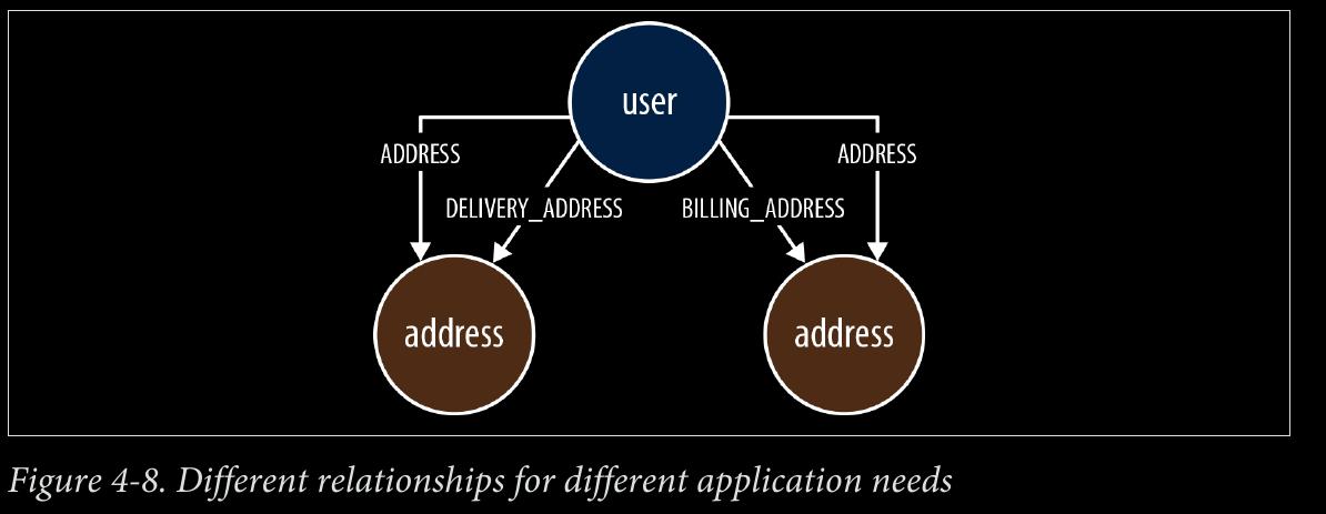
difference between using DELIVERY_ADDRESS and HOME_ADDRESS versus ADDRESS {type: ‘delivery’} and ADDRESS {type: ‘home’}.
-
Sometimes, however, we have a closed set of relationships, but in some traversals we want to follow specific kinds of relationships within that set, whereas in others we want to follow all of them, irrespective of type. Addresses are a good example. Following the closed-set principle, we might choose to create HOME_ADDRESS, WORK_ADDRESS, and DE LIVERY_ADDRESS relationships. This allows us to follow specific kinds of address rela‐ tionships (DELIVERY_ADDRESS, for example) while ignoring all the rest. But what do we do if we want to find all addresses for a user? There are a couple of options here. First, we can encode knowledge of all the different relationship types in our queries: e.g., MATCH user-[:HOME_ADDRESS|WORK_ADDRESS|DELIVERY_ADDRESS]->address. This, however, quickly becomes unwieldy when there are lots of different kinds of relation‐ ships. Alternatively, we can add a more generic ADDRESS relationship to our model, in addition to the fine-grained relationships. Every node representing an address is then connected to a user using two relationships: a fined-grained relationship (e.g., DELIVERY_ADDRESS) and the more generic ADDRESS {type: ‘delivery’} relationship.
-
[:ADDRESS {type:‘delivery’}] OR [:DELIVERY_ADDRESS] OR BOTH
-
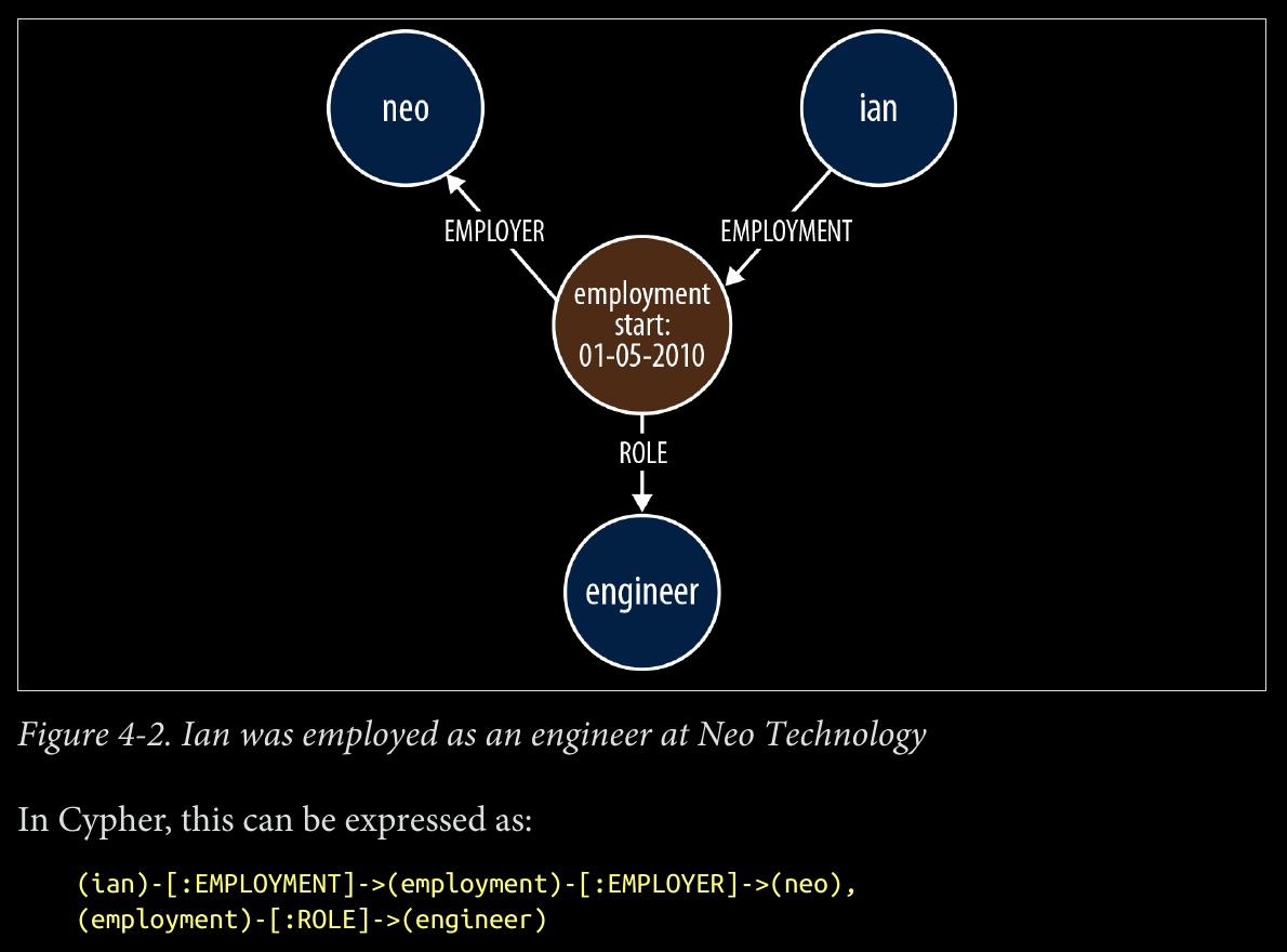
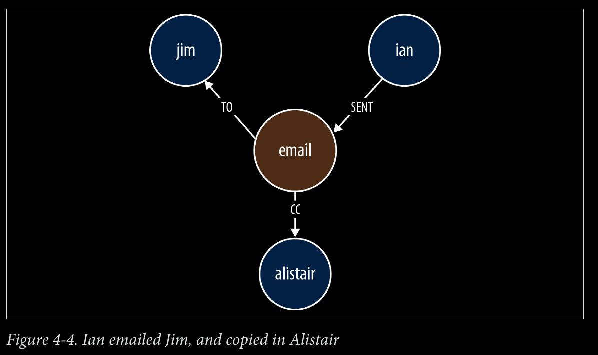
When two or more domain entities interact for a period of time, a fact emerges. We represent these facts as separate nodes, with connections to each of the entities engaged in that fact.
page 69:
- Value types are things that do not have an identity, and whose equivalence is based solely on their values. Examples include money, address, and SKU. Complex value types are value types with more than one field or property. Address, for example, is a complex value type. Such multiproperty value types are best represented as separate nodes:
START ord=node:orders(orderid={orderId})
MATCH (ord)-[:DELIVERY_ADDRESS]->(address)
RETURN address.first_line, address.zipcode
page 71:
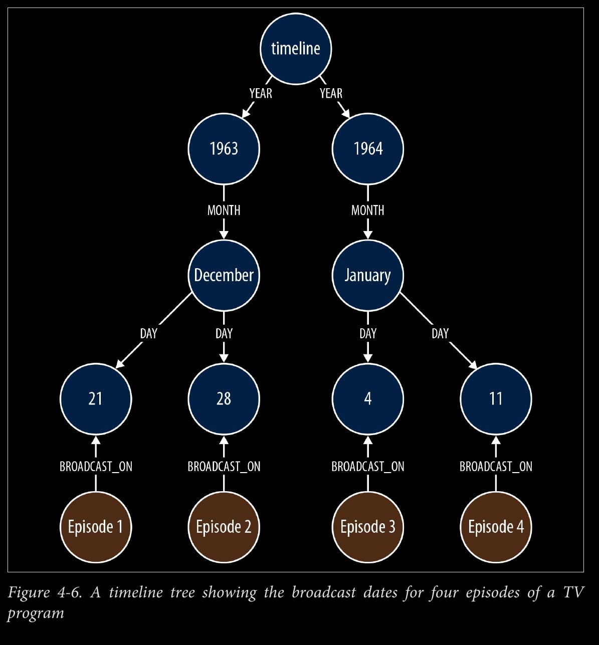
- the following Cypher statement will insert all necessary nodes for a particular event—year, month, day, plus the node representing the event to be attached to the timeline:
START timeline=node:timeline(name={timelineName})
CREATE UNIQUE (timeline)-[:YEAR]->(year{value:{year}, name:{yearName}})
              -[:MONTH]->(month{value:{month}, name:{monthName}})
              -[:DAY]->(day{value:{day}, name:{dayName}})
              <-[:BROADCAST_ON]-(n {newNode})
- Querying the calendar for all events between a start date (inclusive) and an end date (exclusive) can be done with the following Cypher:
START timeline=node:timeline(name={timelineName})
MATCH (timeline)-[:YEAR]->(year)-[:MONTH]->(month)-[:DAY]->
      (day)<-[:BROADCAST_ON]-(n)
WHERE ((year.value > {startYear} AND year.value < {endYear})
      OR ({startYear} = {endYear} AND {startMonth} = {endMonth}
          AND year.value = {startYear} AND month.value = {startMonth}
          AND day.value >= {startDay} AND day.value < {endDay})
      OR ({startYear} = {endYear} AND {startMonth} < {endMonth}
          AND year.value = {startYear}
          AND ((month.value = {startMonth} AND day.value >= {startDay})
              OR (month.value > {startMonth} AND month.value < {endMonth})
              OR (month.value = {endMonth} AND day.value < {endDay})))
      OR ({startYear} < {endYear}
          AND year.value = {startYear}
          AND ((month.value > {startMonth})
              OR (month.value = {startMonth} AND day.value >= {startDay})))
      OR ({startYear} < {endYear}
          AND year.value = {endYear}
          AND ((month.value < {endMonth})
              OR (month.value = {endMonth} AND day.value < {endDay}))))
RETURN n
-
The WHERE clause here, though somewhat verbose, simply filters each match based on the start and end dates supplied to the query.
-
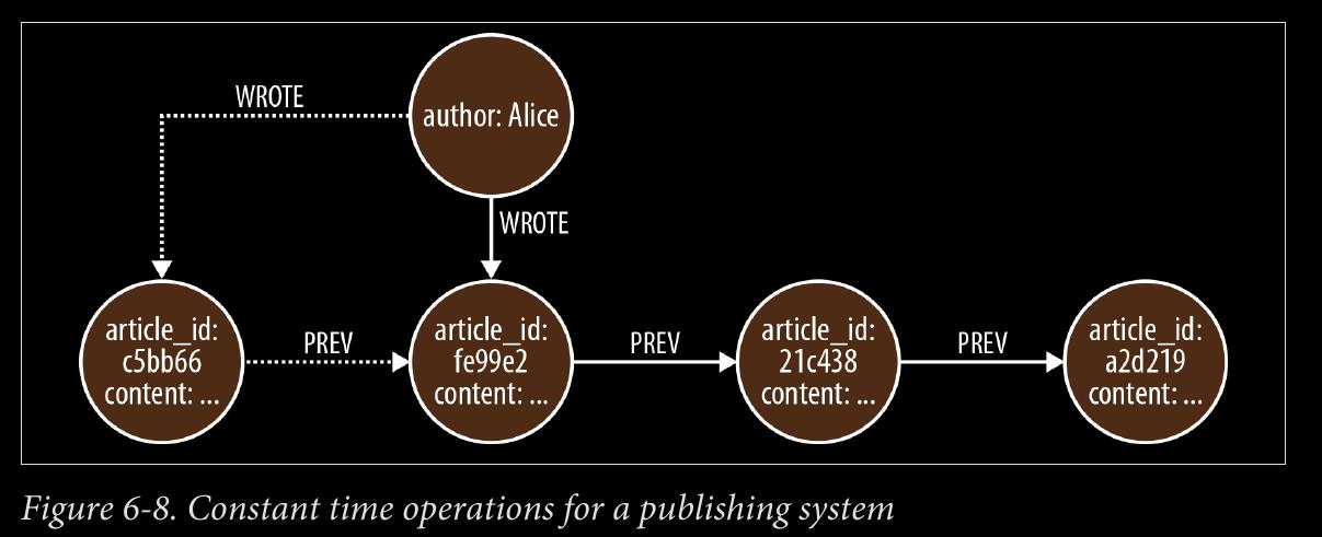
We can use NEXT and PREVIOUS relationships (or similar) to create linked lists that cap‐ ture this natural ordering, as shown in Figure 4-7. Linked lists allow for very rapid traversal of time-ordered events.
page 72:
-
can be versioned with timestamps, but complexity leaks into queries
-
example, github.com/dmontag/neo4j-versioning, which uses Neo4j’s transaction life cycle to create versioned copies of nodes and relationships.
-
different relationships can sit side-by-side with one another, catering to different needs without distorting the model in favor of any one particular need.
-
Start with some of the model and then add to it as needed, much like the iterative software development cycle most use.
-
Being able to add new relationships to meet new application needs doesn’t mean we should always do this. We’ll invariably identify opportunities for refactoring the model as we go: there’ll be plenty of times, for example, where renaming an existing relation‐ ship will allow it to be used for two different needs. When these opportunities arise, we should take them. If we’re developing our solution in a test-driven manner—described in more detail later in this chapter—we’ll have a sound suite of regression tests in place, enabling us to make substantial changes to the model with confidence.
page 83:
- With test-driven data modeling, we write unit tests based on small, representative ex‐ ample graphs drawn from our domain. These example graphs contain just enough data to communicate a particular feature of the domain; in many cases, they might only comprise 10 or so nodes, plus the relationships that connect them. We use these examples to describe what is normal for the domain, and also what is exceptional.
page 85:
-
ImpermanentGraphDatabase, which is a lightweight, in-memory version of Neo4j designed specifically for unit testing. By using ImpermanentGraphDatabase, we avoid having to clear up store files on disk after each test.
-
ImpermanentGraphDatabase should only be used in unit tests. It is not a production-ready, in-memory version of Neo4j.
page 89:
-
When creating query performance tests, bear in mind the following guidelines:
-
Create a suite of performance tests that exercise the queries developed through our unit testing. Record the performance figures so that we can see the relative effects of tweaking a query, modifying the heap size, or upgrading from one version of a graph database to another. Testing
-
Run these tests often, so that we quickly become aware of any deterioration in performance. We might consider incorporating these tests into a continuous de‐ livery build pipeline, failing the build if the test results exceed a certain value.
-
Run these tests in-process on a single thread. There’s no need to simulate multiple clients at this stage: if the performance is poor for a single client, it’s unlikely to improve for multiple clients. Even though they are not, strictly speaking, unit tests, we can drive them using the same unit testing framework we use to develop our unit tests.
-
Run each query many times, picking starting nodes at random each time, so that we can see the effect of starting from a cold cache, which is then gradually warmed as multiple queries execute.
page 91:
- When creating a representative dataset, we try to reproduce any domain invariants we have identified: the minimum, maximum, and average number of relationships per node, the spread of different relationship types, property value ranges, and so on.
page 92:
- Representative datasets also help with capacity planning. Whether we create a full-sized dataset, or a scaled-down sample of what we expect the production graph to be, our representative dataset will give us some useful figures for estimating the size of the production data on disk.
page 94:
- Spinning disk is by far the slowest part of the database stack. Queries that have to reach all the way down to spinning disk will be orders of magnitude slower than queries that touch only the object cache. Disk access can be improved by using solid-state drives (SSDs) in place of spinning disks, providing an approximate 20 times increase in performance
page 95:
-
There are, then, three areas in which we can optimize for performance:
-
Increase the object cache (from 2 GB, all the way up to 200 GB or more in exceptional circumstances)
-
Increase the percentage of the store mapped into the filesystem cache
-
Invest in faster disks: SSDs or enterprise flash hardware
-
The first two options here require adding more RAM. In costing the allocation of RAM, however, there are a couple of things to bear in mind. First, whereas the size of the store files in the filesystem cache map one-to-one with the size on disk, graph objects in the object cache can be up to 10 times bigger than their on-disk representations. Allocating RAM to the object cache is, therefore, far more expensive per graph element than allo‐ cating it to the filesystem cache. The second point to bear in mind relates to the location of the object cache. If our graph database uses an on-heap cache, as does Neo4j, then increasing the size of the cache requires allocating more heap. Most modern JVMs do not cope well with heaps much larger than 8 GB. Once we start growing the heap beyond this size, garbage collection can impact the performance of our application. [8]
-
[8] Neo4j Enterprise Edition includes a cache implementation that mitigates the problems encountered with large heaps, and is being successfully used with heaps in the order of 200 GB.

CHAPTER 5 - Graphs in the Real World
- useful real world examples
page 103:
-
The distinction between network management of a large communications network versus data center manage‐ ment is largely a matter of which side of the firewall you’re working. For all intents and purposes, these two things are one and the same.
-
visualize the network
-
Which parts of the network—which applications, services, virtual machines, phys‐ ical machines, data centers, routers, switches, and fibre—do important customers depend on? (Top-down analysis)
-
Conversely, which applications and services, and ultimately, customers, in the net‐ work will be affected if a particular network element—a router or switch, for ex‐ ample—fails? (Bottom-up analysis)
-
Is there redundancy throughout the network for the most important customers?
page 104:
-
access control and authorization
-
custom SQL solutions can’t grow big
-
As with network management and analysis, a graph database access control solution allows for both top-down and bottom-up queries:
-
Which resources—company structures, products, services, agreements, and end users—can a particular administrator manage? (Top-down)
-
Which resource can an end user access?
-
Given a particular resource, who can modify its access settings? (Bottom-up)
page 111:
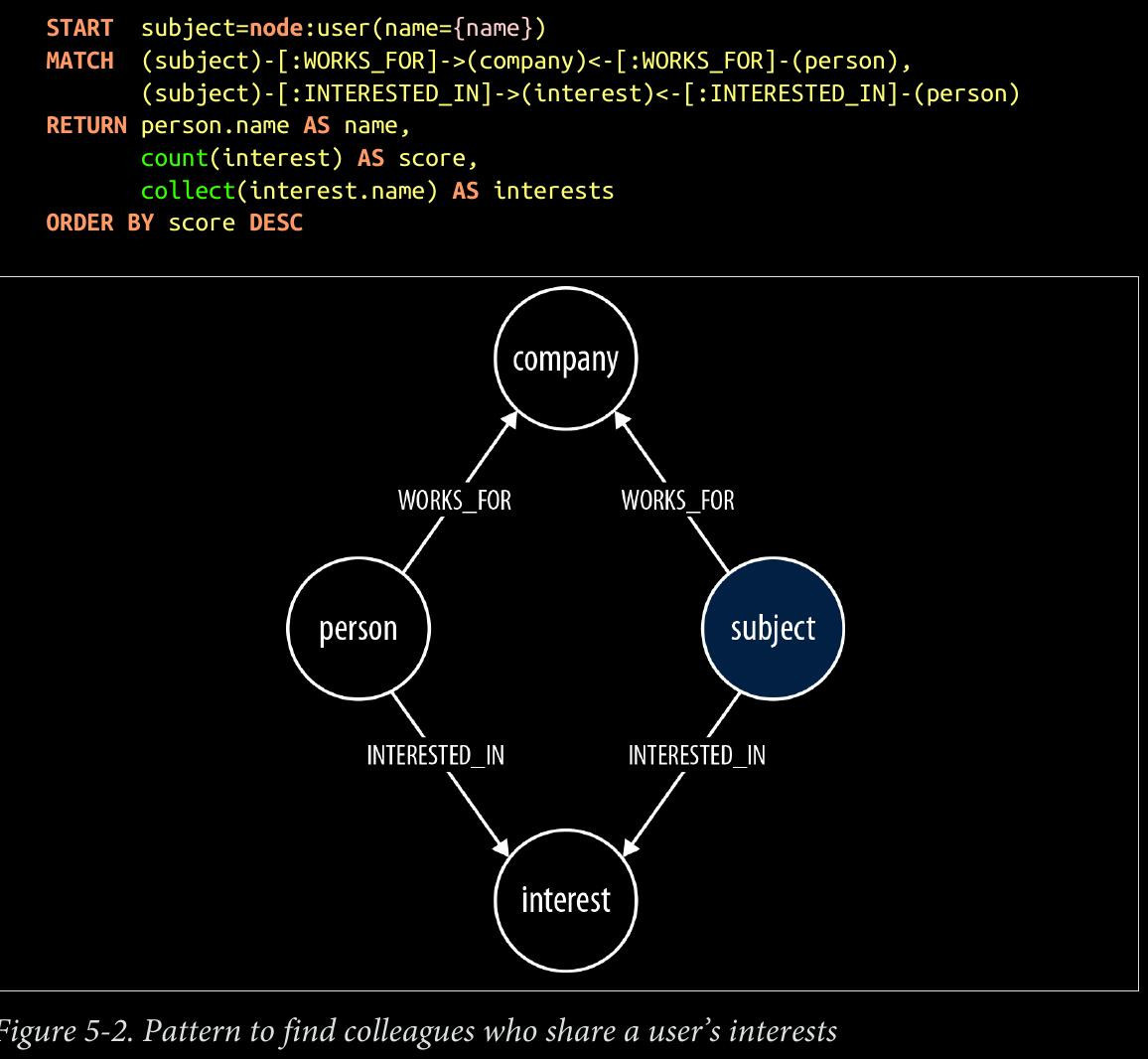
MATCH p=(subject)-[:WORKED_ON]->()-[:WORKED_ON*0..2]-()
      <-[:WORKED_ON]-(person)-[:INTERESTED_IN]->(interest)
page 112:
- The MATCH clause in the preceding query uses a variable-length path, [:WORKED_ON*0..2], as part of a larger pattern to match people who have worked di‐ rectly with the subject of the query, as well as people who have worked on the same project as people who have worked with the subject. Because each person is separated from the subject of the query by one or two pairs of WORKED_ON relationships, Talent.net could have written this portion of the query as MATCH p=(subject)- [:WORKED_ON*2..4]-(person)-[:INTERESTED_IN]->(interest), with a variable- length path of between two and four WORKED_ON relationships. However, long variable- length paths can be relatively inefficient. When writing such queries, it is advisable to restrict variable-length paths to as narrow a scope as possible. To increase the perfor‐ mance of the query, Talent.net uses a fixed-length outgoing WORKED_ON relationship that extends from the subject to her first project, and another fixed-length WORKED_ON rela‐ tionship that connects the matched person to a project, with a smaller variable-length path in between.
page 117:
-
interesting
-
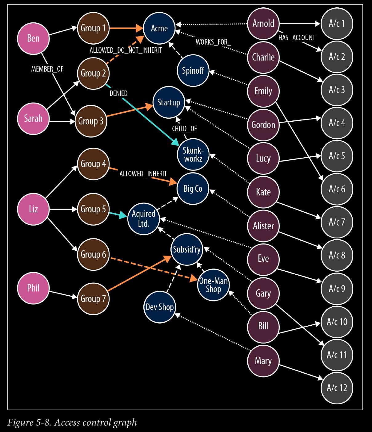
ALLOWED_INHERIT connects an administrator group to an organizational unit, thereby allowing administrators within that group to manage the organizational unit. This permission is inherited by children of the parent organizational unit. We see an example of inherited permissions in the TeleGraph example data model in the relationships between Group 1 and Acme, and the child of Acme, Spinoff. Group 1 is connected to Acme using an ALLOWED_INHERIT relationship. Ben, as a member of Group 1, can manage employees both of Acme and Spinoff thanks to this AL LOWED_INHERIT relationship.
page 118:
-
ALLOWED_DO_NOT_INHERIT connects an administrator group to an organizational unit in a way that allows administrators within that group to manage the organi‐ zational unit, but not any of its children. Sarah, as a member of Group 2, can ad‐ minister Acme, but not its child Spinoff, because Group 2 is connected to Acme by an ALLOWED_DO_NOT_INHERIT relationship, not an ALLOWED_INHERIT relationship.
-
access control graph
page 119:
-
DENIED forbids administrators from accessing an organizational unit. This permis‐ sion is inherited by children of the parent organizational unit. In the TeleGraph diagram, this is best illustrated by Liz and her permissions with respect to Big Co, Acquired Ltd, Subsidiary, and One-Map Shop . As a result of her membership of Group 4 and its ALLOWED_INHERIT permission on Big Co , Liz can manage Big Co. But despite this being an inheritable relationship, Liz cannot manage Acquired Ltd or Subsidiary; the reason being, Group 5, of which Liz is a member, is DE NIED access to Acquired Ltd and its children (which includes Subsidiary). Liz can, however, manage One-Map Shop, thanks to an ALLOWED_DO_NOT_INHERIT per‐ mission granted to Group 6, the last group to which Liz belongs.
-
DENIED takes precedence over ALLOWED_INHERIT, but is subordinate to AL LOWED_DO_NOT_INHERIT. Therefore, if an administrator is connected to a company by way of ALLOWED_DO_NOT_INHERIT and DENIED, ALLOWED_DO_NOT_INHERIT prevails.
-
Notice that the TeleGraph access control data model uses fine-grained relationships (ALLOWED_INHERIT, ALLOWED_DO_NOT_INHERIT, and DENIED) rather than a single rela‐ tionship type qualified by properties—something like PERMISSION with allowed and inherited boolean properties. TeleGraph performance-tested both approaches and determined that the fine-grained, property-free approach was nearly twice as fast as the one using properties.
-
ability to find all the resources an administrator can access… results returned from the following query:
START admin=node:administrator(name={administratorName})
MATCH paths=(admin)-[:MEMBER_OF]->()-[:ALLOWED_INHERIT]->()
      <-[:CHILD_OF*0..3]-(company)<-[:WORKS_FOR]-(employee)
      -[:HAS_ACCOUNT]->(account)
WHERE NOT ((admin)-[:MEMBER_OF]->()-[:DENIED]->()<-[:CHILD_OF*0..3]-(company))
RETURN employee.name AS employee, account.name AS account
UNION
START admin=node:administrator(name={administratorName})
MATCH paths=(admin)-[:MEMBER_OF]->()-[:ALLOWED_DO_NOT_INHERIT]->()
      <-[:WORKS_FOR]-(employee)-[:HAS_ACCOUNT]->(account)
RETURN employee.name AS employee, account.name AS account
page 120:
-
This query sets the template for all the other queries we’ll be looking at in this section, in that it comprises two separate queries joined by a UNION operator
-
The query before the UNION operator handles ALLOWED_INHERIT relationships qualified by any DENIED relationships; the query following the UNION op‐ erator handles any ALLOWED_DO_NOT_INHERIT permissions. This pattern, ALLOWED_IN HERIT minus DENIED, followed by ALLOWED_DO_NOT_INHERIT, is repeated in all of the access control example queries that follow.
-
The first query here, the one before the UNION operator, can be broken down as follows:
-
START finds the logged-in administrator in the administrator index, and binds the result to the admin identifier.
-
MATCH matches all the groups to which this administrator belongs, and from these groups, all the parent companies connected by way of an ALLOWED_INHERIT rela‐ tionship. The MATCH then uses a variable-length path ([:CHILD_OF*0..3]) to dis‐ cover children of these parent companies, and thereafter the employees and ac‐ counts associated with all matched companies (whether parent company or child). At this point, the query has matched all companies, employees, and accounts ac‐ cessible by way of ALLOWED_INHERIT relationships.
-
WHERE eliminates matches whose company, or parents, are connected by way of DENIED relationship to the administrator’s groups. This WHERE clause is invoked for each match; if there is a DENIED relationship anywhere between the admin node and the company node bound by the match, that match is eliminated.
-
RETURN creates a projection of the matched data in the form of a list of employee names and accounts. The second query here, following the UNION operator, is a little simpler:
-
The MATCH clause simply matches companies (plus employees and accounts) that are directly connected to an administrator’s groups by way of an AL LOWED_DO_NOT_INHERIT relationship.
page 122:
- What’s needed is a query that will determine whether an administrator has access to a specific resource. This is that query:
START admin=node:administrator(name={adminName}),
      company=node:company(resourceName={resourceName})
MATCH p=(admin)-[:MEMBER_OF]->()-[:ALLOWED_INHERIT]->()
      <-[:CHILD_OF*0..3]-(company)
WHERE NOT ((admin)-[:MEMBER_OF]->()-[:DENIED]->()
          <-[:CHILD_OF*0..3]-(company))
RETURN count(p) AS accessCount
UNION
START admin=node:administrator(name={adminName}),
      company=node:company(resourceName={resourceName})
MATCH p=(admin)-[:MEMBER_OF]->()-[:ALLOWED_DO_NOT_INHERIT]->(company)
RETURN count(p) AS accessCount
-
This query works by determining whether an administrator has access to the company to which an employee or an account belongs. How do we identify the company to which an employee or account belongs? Through clever use of indexes.
-
In the TeleGraph data model, companies are indexed both by their name, and by the names of their employees and employee accounts. Given a company name, employee name, or account name, we can, therefore, look up the relevant company node in the company index.
-
With that bit of insight, we can see that this resource authorization check is similar to the query for finding all companies, employees, and accounts—only with several small differences:
-
company is bound in the START clause, not the MATCH clause. Using the indexing strategy described earlier, we look up the node representing the relevant company based on the name of the resource to be authorized—whether employee or account.
-
We don’t match any further than company. Because company has already been bound based on an employee or account name, there’s no need to drill further into the graph to match that employee or account.
-
The RETURN clauses for the queries before and after the UNION operator return a count of the number of matches. For an administrator to have access to a resource, one or both of these accessCount values must be greater than 0.
page 123:
- The previous two queries represent “top-down” views of the graph. The last TeleGraph query we’ll discuss here provides a “bottom-up” view of the data. Given a resource—an employee or account—who can manage it? Here’s the query:
START resource=node:resource(name={resourceName})
MATCH p=(resource)-[:WORKS_FOR|HAS_ACCOUNT*1..2]-(company)
      -[:CHILD_OF*0..3]->()<-[:ALLOWED_INHERIT]-()<-[:MEMBER_OF]-(admin)
WHERE NOT ((admin)-[:MEMBER_OF]->()-[:DENIED]->()<-[:CHILD_OF*0..3]-(company))
RETURN admin.name AS admin
UNION
START resource=node:resource(name={resourceName})
MATCH p=(resource)-[:WORKS_FOR|HAS_ACCOUNT*1..2]-(company)
      <-[:ALLOWED_DO_NOT_INHERIT]-()<-[:MEMBER_OF]-(admin)
RETURN admin.name AS admin
-
The START clauses use a resource index, a named index for both employees and accounts.
-
The MATCH clauses contain a variable-length path expression that uses the | operator to specify a path that is one or two relationships deep, and whose relationship types comprise WORKS_FOR and HAS_ACCOUNT. This expression accommodates the fact that the subject of the query may be either an employee or an account.
page 132:
-
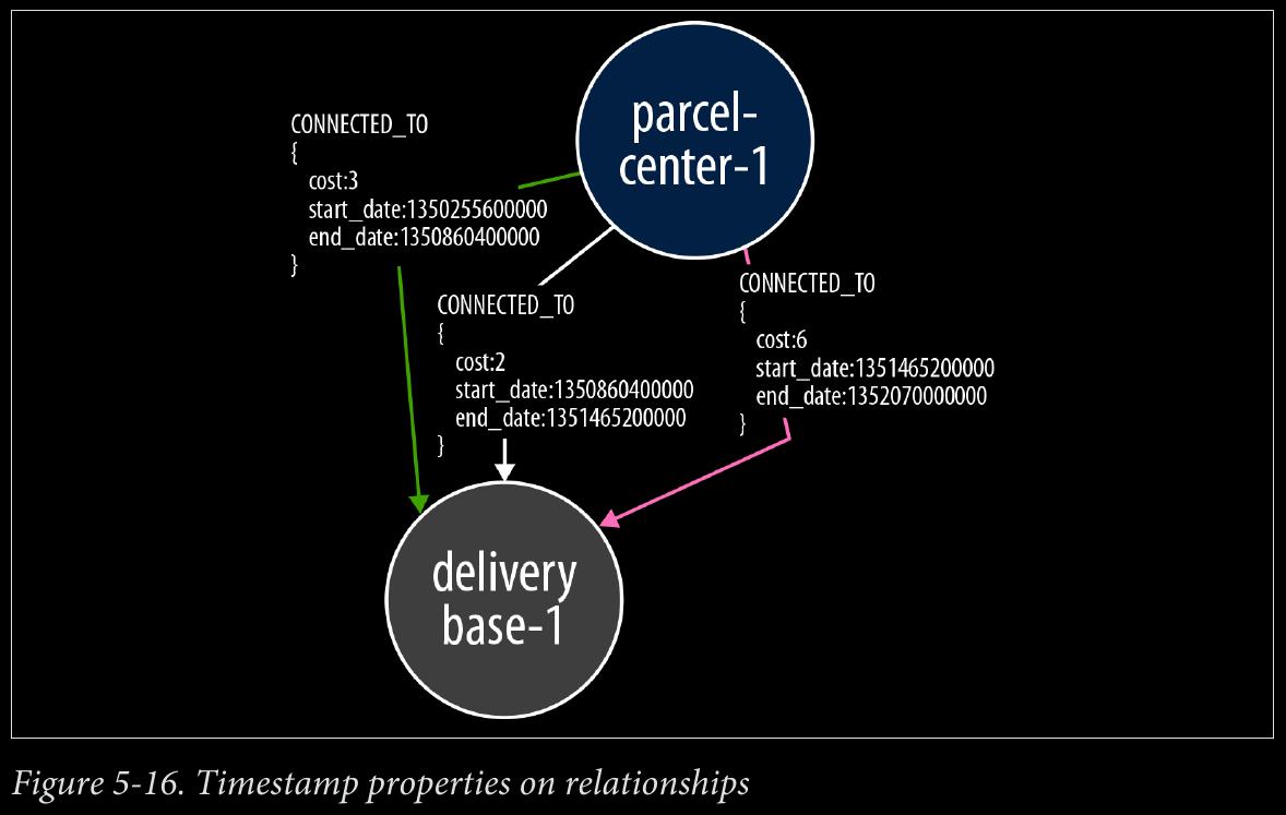
The Cypher query to implement the parcel route calculation engine
-
4 smaller queries WITH’d together
CHAPTER 6 - Graph Database Internals
page 141:
-
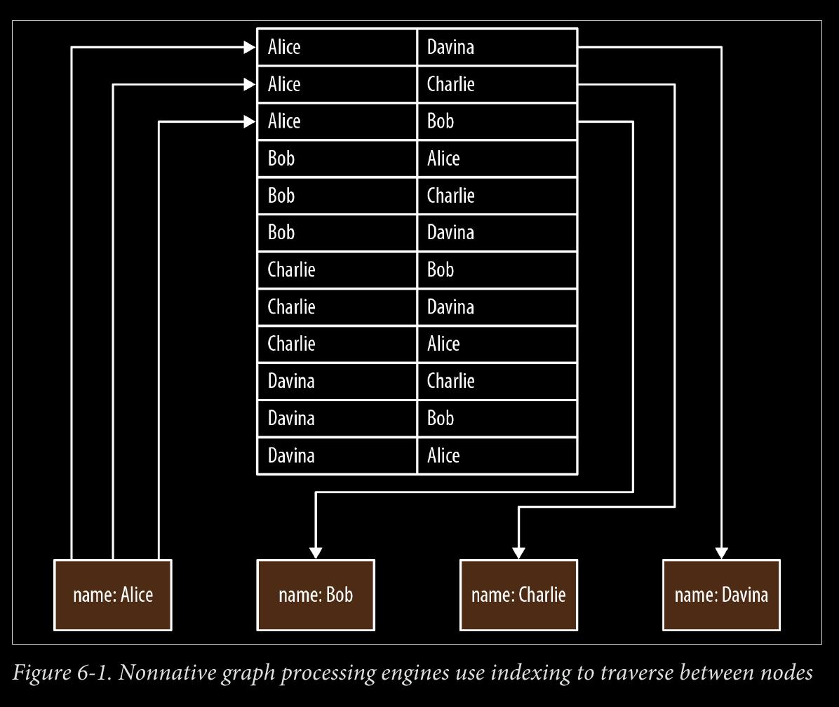
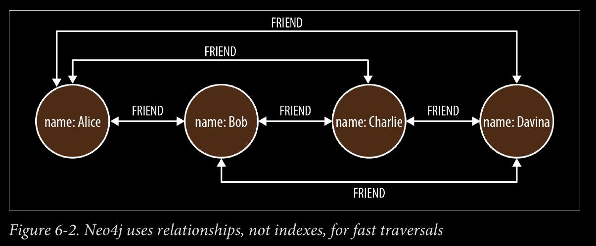
we say that a graph database has native processing capabilities if it exhibits a property called index-free adjacency.
-
A database engine that utilizes index-free adjacency is one in which each node maintains direct references to its adjacent nodes; each node, therefore acts as a micro-index of other nearby nodes, which is much cheaper than using global indexes. It means that query times are independent of the total size of the graph, and are instead simply pro‐ portional to the amount of the graph searched.
page 142:
- To understand why native graph processing is so much more efficient than graphs based on heavy indexing, consider the following. Depend‐ ing on the implementation, index lookups could be O(log n) in algo‐ rithmic complexity versus O(1) for looking up immediate relationships. To traverse a network of m steps, the cost of the indexed approach, at O(m log n), dwarfs the cost of O(m) for an implementation that uses index-free adjacency.
page 143:
- With index-free adjacency, bidirectional joins are effectively precomputed and stored in the database as relationships. In contrast, when using indexes to fake connections between records, there is no actual relationship stored in the database. This becomes problematic when we try to traverse in the “opposite” direction from the one for which the index was constructed. Because we have to perform a brute-force search through the index—which is an O(n) operation—joins like this are simply too costly to be of any practical use.
page 150:
- these APIs can be thought of as a stack, as depicted in Figure 6-7: at the top we prize expressiveness and declarative programming; at the bottom we prize precision, imperative style, and (at the lowest layer) “bare metal” performance.

CHAPTER 7 - Predictive Analysis with Graph Theory
page 165:
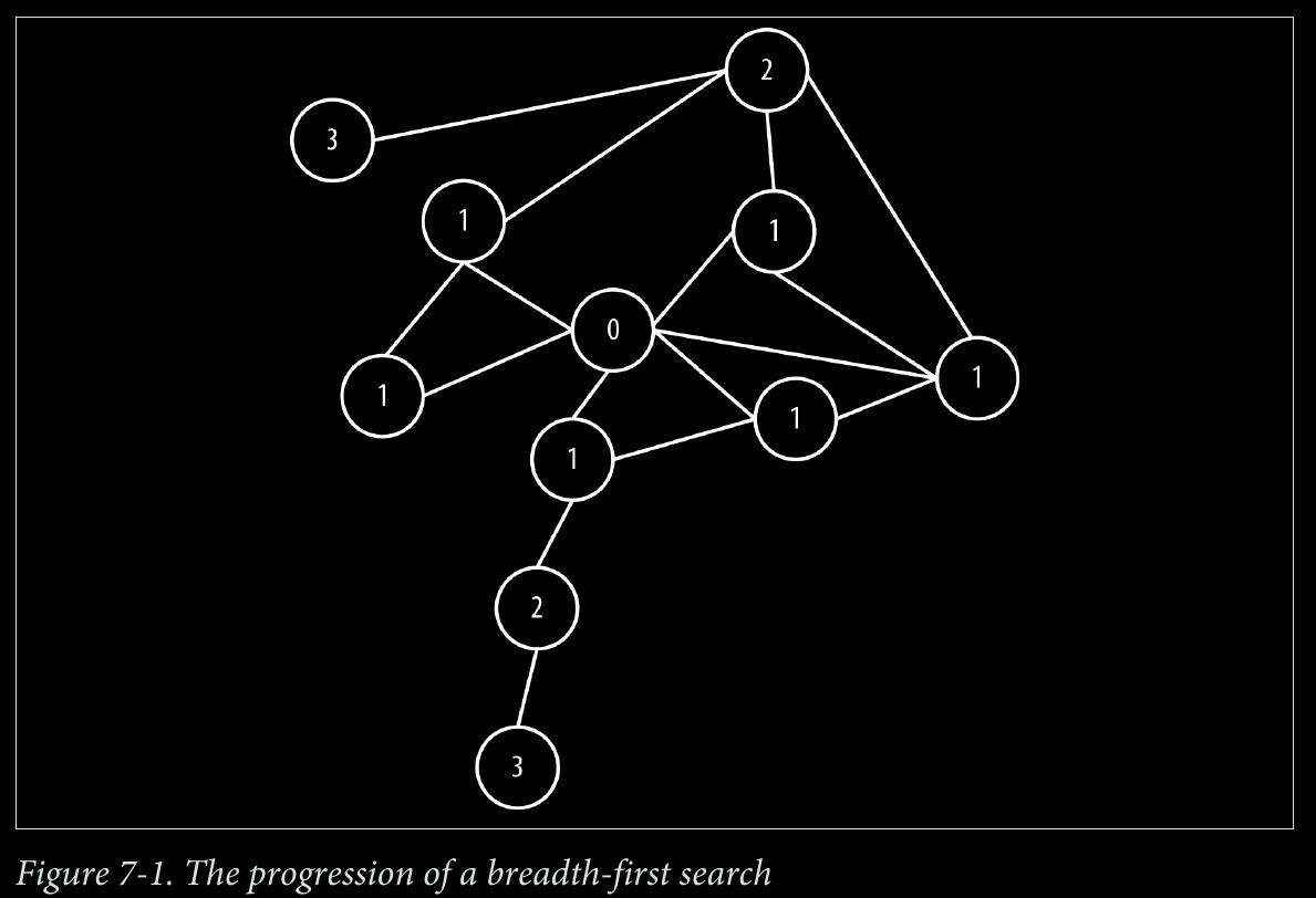
- Dijkstra’s algorithm is mature, having been published in 1956, and thereafter widely studied and optimized by computer scientists. It behaves as follows:
-
Pick the start and end nodes, and add the start node to the set of solved nodes (that is, the set of nodes with known shortest path from the start node) with value 0 (the start node is by definition 0 path length away from itself).
-
From the starting node, traverse breadth-first to the nearest neighbors and record the path length against each neighbor node.
-
Take the shortest path to one of these neighbors (picking arbitrarily in the case of ties) and mark that node as solved, because we now know the shortest path from the start node to this neighbor.
-
From the set of solved nodes, visit the nearest neighbors (notice the breath-first progression) and record the path lengths from the start node against these new neighbors. Don’t visit any neighboring nodes that have already been solved, because we know the shortest paths to them already.
-
Repeat steps 3 and 4 until the destination node has been marked solved. Efficiency of Dijkstra’s Algorithm Dijkstra’s algorithm is quite efficient because it computes only the lengths of a relatively small subset of the possible paths through the graph. When we’ve solved a node, the shortest path from the start node is then known, allowing all subsequent paths to safely build on that knowledge.
-
In fact, the fastest known worst-case implementation of Dijkstra’s algorithm has a per‐ formance of O(|R| + |N| log |N|). That is, the algorithm runs in time proportional to the number of relationships in the graph, plus the size of the number of nodes multiplied by the log of the size of the node set. The original was O(|R|^2), meaning it ran in time proportional to the square of the size of the number of relationships in the graph.
-
Dijkstra is often used to find real-world shortest paths (e.g., for navigation). Here’s an example.
page 173:
- A* is both like Dijkstra in that it can potentially search a large swathe of a graph, but it’s also like a greedy best-first search insofar as it uses a heuristic to guide it. A* combines aspects of Dijkstra’s algorithm, which prefers nodes close to the current starting point, and best-first search, which prefers nodes closer to the destination, to provide a provably optimal solution for finding shortest paths in a graph. In A* we split the path cost into two parts: g(n), which is the cost of the path from the starting point to some node n; and h(n), which represents the estimated cost of the path from the node n to the destination node, as computed by a heuristic (an intelligent guess). The A* algorithm balances g(n) and h(n) as it iterates the graph, thereby ensuring that at each iteration it chooses the node with the lowest overall cost f(n) = g(n) + h(n).
page 175:
-
A triadic closure is a common property of social graphs, where we observe that if two nodes are connected via a path involving a third node, there is an increased likelihood that the two nodes will become directly connected at some point in the future. This is a familiar social occurrence: if we happen to be friends with two people, there’s an increased chance that those people will become direct friends too. The very fact of their both being our friend is an indicator that with respect to each other they may be socially similar.
-
From his analysis, Granovetter noted that a subgraph upholds the strong triadic closure property if it has a node A with strong relationships to two other nodes, B and C. B and C then have at least a weak, and potentially a strong, relationship between them. This is a bold assertion, and it won’t always hold for all subgraphs in a graph. Nonetheless, it is sufficiently commonplace, particularly in social networks, as to be a credible predictive indicator.
page 179:
-
A structurally balanced triadic closure consists of relation‐ ships of all strong sentiments (our WORKS_WITH or PEER_OF relationships) or two rela‐ tionships have negative sentiments (MANAGES in our case) with a single positive rela‐ tionship.
-
We see this often in the real world. If we have two good friends, then social pressure tends toward those good friends themselves becoming good friends. It’s unusual that those two friends themselves are enemies because that puts a strain on our friendships. One friend cannot express his dislike of the other to us, because the other person is our friend too! Given those pressures, it’s reasonably likely that ultimately the group will resolve its differences and good friends will emerge.
-
This would change our unbalanced triadic closure (two relationships with positive sen‐ timents and one negative) to a balanced closure because all relationships would be of a positive sentiment much like our collaborative scheme where Alice, Bob, and Charlie all work together in Figure 7-18.
page 180:
-
However, another plausible (though arguably less pleasant) outcome would be where we take sides in the dispute between our “friends” creating two relationships with neg‐ ative sentiments—effectively ganging up on an individual. Now we can engage in gossip about our mutual dislike of a former friend and the closure again becomes balanced. Equally we see this reflected in the organizational scenario where Alice, by managing Bob and Charlie, becomes, in effect, their workplace enemy as in Figure 7-17.
-
local bridges
APPENDIX A - NOSQL: Overview
page 185:
- The ACID guarantees provide us with a safe environment in which to operate on data: {% endfilter %}
{% filter markdown %}
-
Atomic - All operations in a transaction succeed or every operation is rolled back.
-
Consistent - On transaction completion, the database is structurally sound.
-
Isolated - Transactions do not contend with one another. Contentious access to state is mod‐ erated by the database so that transactions appear to run sequentially.
-
Durable - The results of applying a transaction are permanent, even in the presence of failures {% endfilter %}
{% filter markdown %}
- BASE {% endfilter %}
{% filter markdown %}
-
Basic availability - The store appears to work most of the time.
-
Soft-state - Stores don’t have to be write-consistent, nor do different replicas have to be mutually consistent all the time.
-
Eventual consistency - Stores exhibit consistency at some later point (e.g., lazily at read time). {% endfilter %}
{% filter markdown %}
-
The BASE properties are considerably looser than the ACID guarantees, and there is no direct mapping between them.
-
Graphs use ACID
page 186:
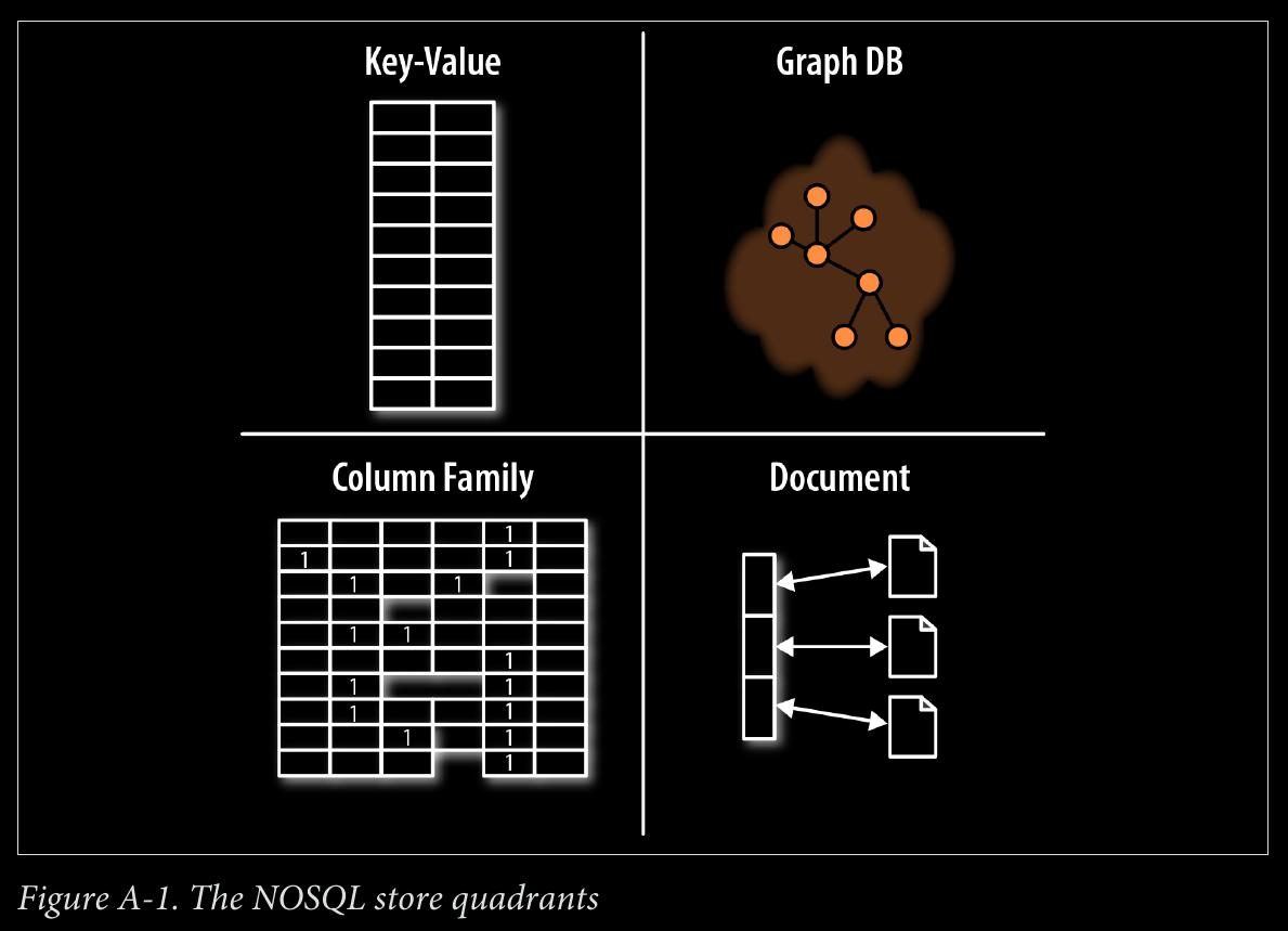
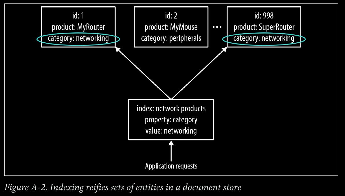
- document stores
page 189:
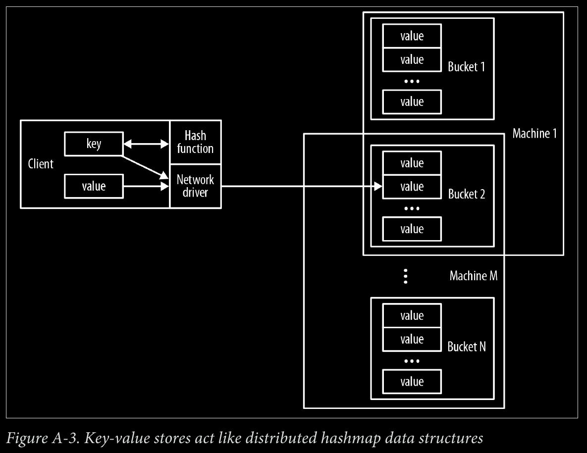
- key-value stores
page 192:
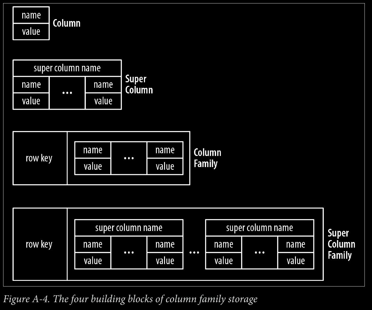
- column family stores
page 193:
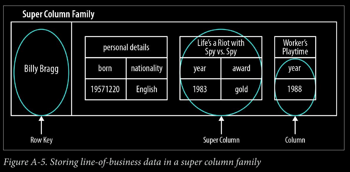
- super column family structure—logically, it’s really nothing more than maps of maps.
page 196:
-
Two properties of graph databases are useful to understand when investigating graph database technologies:
-
The underlying storage - Some graph databases use native graph storage, which is optimized and designed for storing and managing graphs. Not all graph database technologies use native graph storage, however. Some serialize the graph data into a relational database, object-oriented databases, or other types of general-purpose data stores.
-
The processing engine - Some definitions of graph databases require that they be capable of index-free adjacency, meaning that connected nodes physically “point” to each other in the database. Here we take a slightly broader view: that any database that from the user’s perspective behaves like a graph database (i.e., exposes a graph data model through CRUD operations), qualifies as a graph database. We do acknowledge, however, the significant performance advantages of index-free adjacency, and therefore use the term native graph processing in reference to graph databases that leverage index- free adjacency.
